
Tabular and Time Series Foundation Models in 2026: A Research Plan for Mitra-v2, TimesFM, TimeH2O and the Databases That Feed Them
The top 11 single-model entries on GIFT-Eval are within 5% on MASE. On one series, history length changed which of TimesFM 2.5 and Chronos-2 had the lower mean error. A plan to test context policy for Mitra-v2 and forecasters, plus the database caps that set it.
Tabular and Time Series Foundation Models in 2026: A Research Plan for Mitra-v2, TimesFM, TimeH2O and the Databases That Feed Them
Table of Contents
- Key Takeaways
- What to Do on Monday
- Why a Research Plan Now
- The Models: Mitra-v2, TimesFM, TimeH2O and Their Peers
- What the Leaderboards Say When You Recompute Them
- The Hypothesis: Context Policy Versus Model Choice
- Pilot Results for Tabular and Time Series Foundation Models
- Databases That Feed Time Series Foundation Models
- Advanced Data Patterns for Model Context
- The Research Plan
- Frequently Asked Questions
- Conclusion
- References and Further Reading
Between late August and mid-November 2026, Google, Amazon and H2O.ai released new tabular and time series foundation models: TimesFM 3.0, Mitra-v2 and TimeH2O. In the same weeks, IBM and Confluent put Granite time series models behind a Flink SQL function, and AWS added time series collections and managed ingestion to the next generation of Amazon OpenSearch Serverless.
A foundation model for structured data predicts from whatever is placed in its context: labeled rows for a tabular model, recent history for a forecaster. This post calls the rule that fills that context the context policy: which rows or how much history, how many, how fresh, and which covariates (other series or columns that help predict the target). Tabular papers call that input the support set, and forecasting papers call it the history or the context window. In zero-shot use the checkpoint stays fixed. The context policy is set by whoever builds the data platform.
Three more terms recur. An origin is a cut point in time: data before it may be used, and data after it is predicted. The cutoff of a context is the newest row it is allowed to contain. A paired difference compares two options on the same origins or the same benchmark tasks.
This post does two things. First, it reviews these models and the databases around them, with every number traced to a primary source or recomputed from raw leaderboard files on November 19, 2026. For the leaderboards that means we reaggregated the submitted results. We did not rerun the leaderboard models. Second, it proposes a research plan around one question: on time-ordered operational data, how large is the effect of the context policy, compared with the effect of which model you choose?
We also ran a small pilot on one GPU and one public dataset to check that the plan is feasible. One result we expected: a short history hurt one forecaster badly. Two we did not: the other forecaster gained nothing clear beyond 512 points, and for a small tabular context the newest rows alone gave the highest error of the three policies we tried. This post was researched and drafted by an AI coding agent under human direction, and a note at the end says what was and was not run.
Key Takeaways
- The leaders are close, and the top of the board is crowded. We reaggregated all 173 GIFT-Eval entries and the fev-bench results from their raw files. Among single models on GIFT-Eval, the first eleven are within 5 percent of each other in MASE (mean absolute scaled error), from 0.637 to 0.667. Their spread in CRPS (continuous ranked probability score, the measure for probabilistic forecasts) is wider: 0.423 to 0.486. Of the ten paired comparisons between TimeH2O-v1 and the others, eight are inconclusive on both measures. On GIFT-Eval, TimeH2O-v1 is about 2 percent ahead of TimesFM 3.0 in MASE and 3 percent in CRPS, and 6 to 10 percent ahead of Chronos-2 and TimesFM 2.5, both released in autumn 2025. On fev-bench it is 3.6 percent ahead of TimesFM 3.0, 6.7 percent ahead of Chronos-2 and 14.9 percent ahead of TimesFM 2.5. These are submitted results that we reaggregated, not models that we reran.
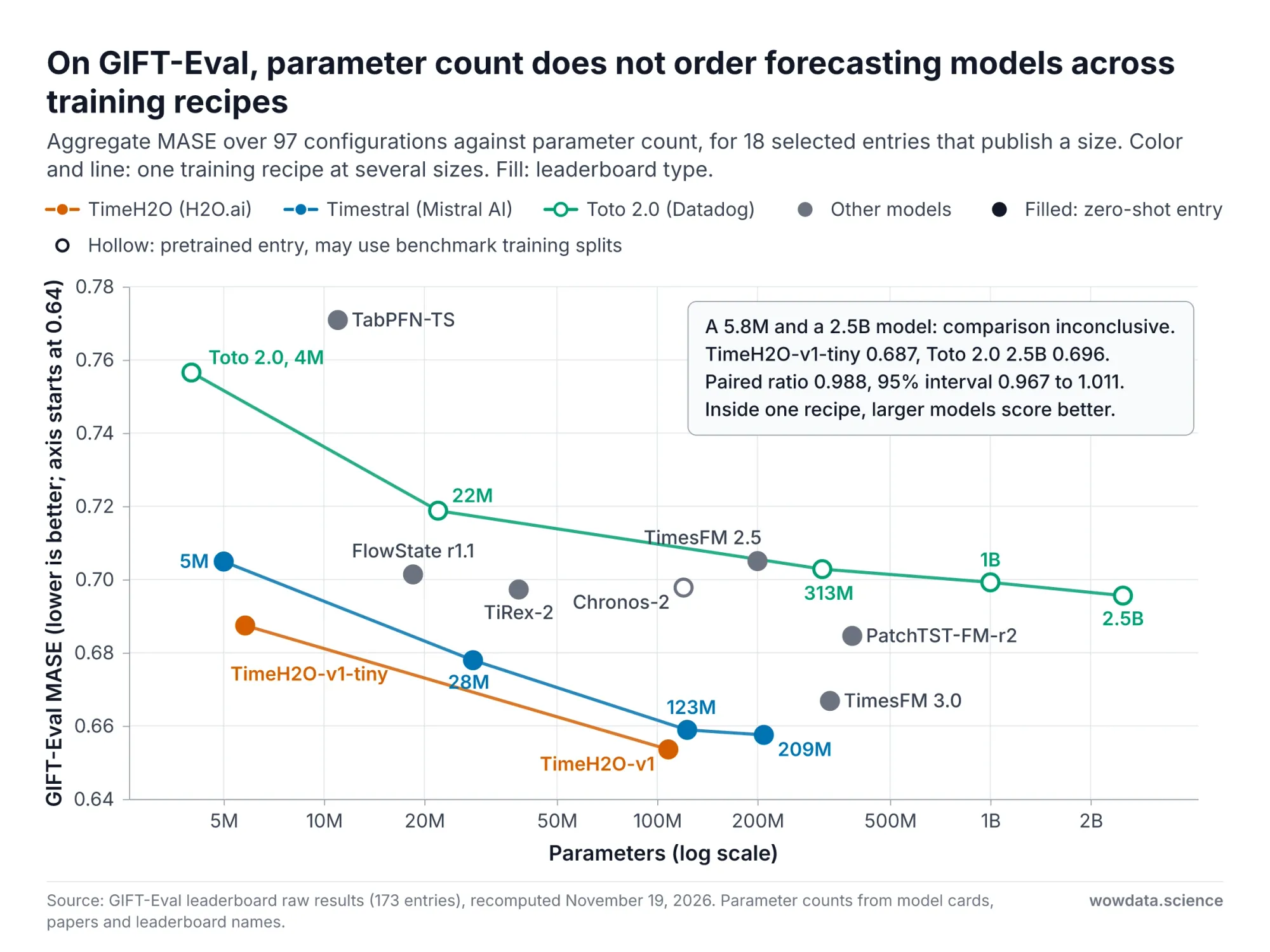
- On GIFT-Eval, parameter count does not order models across training recipes. The 5.8M-parameter TimeH2O-v1-tiny (MASE 0.687) and the 2.5B-parameter Toto 2.0 (0.696) cannot be separated: the ratio of their errors on the same tasks is 0.988, with an interval of 0.967 to 1.011. Within the three families shown, larger variants scored better.
- Amazon reported lower error with larger support sets on the largest TabArena tables. In its sweep, raising Mitra-v2's prediction-time support cap from 512 to 32,768 rows cut error by 28 percent for classification and 21 percent for regression, and 8,192 rows already captured more than 90 percent of that gain. That is one random split per dataset with the fine-tuned recipe, not time-ordered data.
- In our pilot, on one dataset, the largest effects came from short contexts. Given 2,048 points of history instead of 512, Chronos-2's MASE fell from 0.84 to 0.49, and it moved from behind TimesFM 2.5 to ahead of it. For TimesFM 2.5 the same change was inconclusive (0.56 and 0.58). For the zero-shot Mitra-v2 classifier, a context of the newest 512 rows before the origin, used for the three weeks that follow, averaged a log-loss of 0.79, against 0.58 for a uniform sample of history. It was worse at seven of eight origins, which is suggestive and not conclusive.
- Exploratory: freshness helped a context made of recent rows. Advancing the cutoff of the newest-512-rows context every day instead of leaving it at the origin lowered Mitra-v2's mean log-loss from 0.79 to 0.60. The interval just excludes zero and is not adjusted for the many comparisons we made. A mix of new and sampled rows went from 0.58 to 0.49, with an interval that just includes zero. A uniform sample barely changed.
- The pilot is not a test of the hypothesis. Its largest effects came from changing a small support set or extending a short history. It does not show where context stops mattering, or that model choice dominates beyond that point. Those are the questions the plan is built to answer.
- Databases already decide how much context a model gets. Confluent's
AI_FORECASTdefaults to 512 points. BigQuery passes at most 2,048 points to TimesFM 3.0, while the self-hosted weights accept 15,360. OpenSearch Serverless time series collections keep up to ten years of history across hot and warm tiers, but run no forecasting model themselves. - Licenses split the field. Mitra-v2, Chronos-2, TimesFM 2.5 and most IBM Granite models are Apache-2.0. The TimesFM 3.0 and TimeH2O weights are non-commercial.
- The plan. Three research questions, falsifiable hypotheses with contrasts fixed in advance, a rolling-origin design, and a twelve-week schedule on one 24 GB GPU.
What to Do on Monday
Seven things a practitioner can act on now. Each is supported below. The ones marked as pilot results come from one dataset. They are prompts to test, not rules.
- Read the context cap before the model name. Confluent's
AI_FORECASTdefaults to 512 points. BigQuery passes at most 2,048 points to TimesFM 3.0, while the weights accept 15,360. See What Each System Can Express. - Backtest at least two history lengths on your own series before you fix a default. One of two forecasters was clearly better with 2,048 points than with 512. For the other the comparison was inconclusive (pilot, one series). See Pilot 2.
- If a small tabular context cannot be refreshed for weeks, test a sample of history against the newest rows. In the pilot the newest rows alone were worse at seven of eight origins (pilot, one dataset, not conclusive). See Pilot 1.
- If you do use the newest rows, backtest advancing the context cutoff as labels become available. A daily cutoff lowered the error of a newest-rows context (pilot, one dataset, exploratory). See Pilot 1b.
- Check the license before the leaderboard. The TimesFM 3.0 and TimeH2O weights are non-commercial. See the Model Comparison Table.
- Keep both event time and ingestion time on every record, and store the context policy, the refresh time and the model revision with every forecast. Without them you can neither rebuild a context as it was nor evaluate a change later. See Advanced Data Patterns for Model Context.
- Seed or repeat zero-shot Mitra calls. In AutoGluon 1.6.3 the same context gives different probabilities from one call to the next. See Mitra-v2 Classifier and Mitra-v2 Regressor.
Why a Research Plan Now
Three changes affect what is worth testing: new model features, new caps on context, and public benchmark files.
The models changed. TimesFM 3.0 added native multivariate forecasting and covariates. Mitra-v2 extended the context it was pretrained on from 512 to 5,120 rows and replaced its regression head with a predictive distribution. H2O.ai reported TimeH2O-v1, a 108M-parameter model, first of 32 models on fev-bench when it read that leaderboard on October 24. In the benchmark's results on November 17 it is no longer first among the 40 visible entries, as the recomputed tables below show.
The databases changed. Time series collections for the next generation of OpenSearch Serverless arrived on October 28, with a warm storage tier and built-in anomaly detection. Three weeks later, OpenSearch Ingestion could write to them. IBM and Confluent published their streamhouse use cases on November 18, with forecasting as a SQL function over a stream.
The evidence changed too. Two benchmarks built to resist leakage, fev-bench and TIME, now sit beside GIFT-Eval, and their raw results are public. That makes it possible to reaggregate the submitted results and put intervals on vendor claims instead of repeating them.
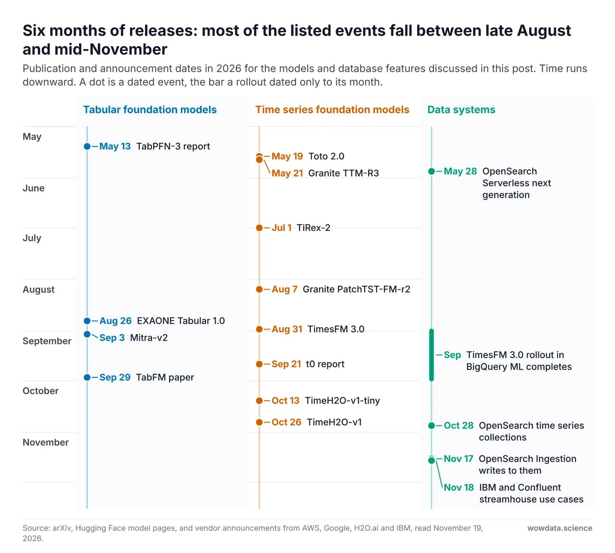
Fig 1: Release timeline for tabular and time series foundation models in 2026 — wowdata.science
The practical question is no longer whether a pretrained model can forecast or classify without training. The open questions are which choices move accuracy on your own time-ordered data, and what your data platform must provide to make those choices possible.
The Models: Mitra-v2, TimesFM, TimeH2O and Their Peers
Mitra-v2 Classifier and Mitra-v2 Regressor
Mitra-v2 is Amazon's second-generation tabular foundation model, released on September 3, 2026, under Apache-2.0 with a technical report and, in November, an Amazon Science article. It comes as two checkpoints: a classifier (75.7M parameters) and a regressor (76.7M). Amazon says the Amazon Connect Customer team led the work and is adopting the model for prediction on structured business data.
A tabular foundation model does not learn weights for your dataset in the usual way. Mitra-v2 was pretrained by Amazon on synthetic prediction tasks. At inference it receives your labeled rows (the support set) and the rows you want predicted (the query) in one forward pass, and it reads the pattern off the support rows. The support set is the model's context, in the same sense as a prompt.
Mitra-v2 is a 12-layer transformer in which every layer attends across rows and then across features. It uses no positional encoding, so its predictions do not depend on the order of rows or columns. That has a consequence for time-ordered data: the model cannot know that one row is newer than another. Time can only enter as a feature, or through the choice of which rows go into the support set.
The 12-layer backbone is unchanged from Mitra-v1. The classifier has the same architecture as its predecessor, and only the regression head is new. The report attributes the gains to the pretraining distribution and the optimizer.
| Component | Mitra-v1 | Mitra-v2 |
|---|---|---|
| Parameters | 75.7M classifier, 75.7M regressor in the report. The v1 model card says 72M | 75.7M classifier, 76.7M regressor |
| Maximum support rows in pretraining | 512 | 5,120 |
| Query rows in pretraining | 128 | 1,280 |
| Maximum features in pretraining | 16 | 50 |
| Synthetic priors | Structural causal models and tree priors | The same, plus a new Hybrid SCM prior |
| Main optimizer | AdamW | Muon |
| Regression head | Single output, mean squared error | 1,000 bins, cross-entropy |
Four details matter for anyone who plans to use it.
The prior is the main design choice. Mitra-v2 is trained only on synthetic data. Most of its prior mass comes from structural causal models: 0.35 from the base prior and 0.35 from a new Hybrid SCM prior that mixes neural networks, trees, 1D convolutions, Gaussian processes and vector autoregression inside one causal graph. Five tree-based generators share the rest.
The regressor returns a distribution. Regression is cast as classification over 1,000 target bins. The point prediction is the mean of that distribution, and the same output gives quantiles and CRPS (continuous ranked probability score). This is the feature that lets a tabular model be scored like a probabilistic forecaster. Amazon reports that the fine-tuned model ranks first on ScoringBench, a benchmark for distributional regression.
The headline numbers are not zero-shot. The reported results use a 50-step fine-tune with 8-fold bagging on a GPU. The report gives a median cost of about 8.8 minutes per evaluation unit for classification and 9.6 minutes for regression, and says the system "should not be described as zero-shot or Pareto-dominant". Amazon's article puts it more gently: "it isn't quite a zero-shot model". The classifier weights can also be used without fine-tuning inside AutoGluon.
Context caps are part of the recipe. The released recipe caps the support set separately for its two phases. Fine-tuning sees at most 16,384 rows for classification and 20,480 for regression. Prediction draws up to 16,384 rows for binary classification, where the subsample is class-balanced, and 32,768 for multiclass classification and regression. When GPU memory runs out it first shrinks the query chunk and then halves the cap, down to 8,192 rows.
We ran both documented paths on an NVIDIA A10G (24 GB) with autogluon.tabular 1.6.3 and mitra-finetune 0.3.0. The zero-shot classifier example from the model card ran as written. The regressor recipe on 2,000 training rows of California housing took 268 seconds end to end and returned RMSE 0.433, CRPS 0.194, and 78.7 percent empirical coverage for its 10 to 90 percent interval.
# Mitra-v2 regressor with a predictive distribution (model card recipe, run on an A10G)
import pandas as pd
from huggingface_hub import snapshot_download
from mitra_finetune import MitraFinetune

ckpt_dir = snapshot_download("autogluon/mitra-regressor-2")
model = MitraFinetune(checkpoint_dir=ckpt_dir, problem_type="regression")
model.fit(X_train, y_train)                    # stores the data
dist = model.predict_distribution(X_test)      # runs the 8-fold bagged fine-tune, then predicts

point = dist.point_prediction                  # mean of the 1,000-bin distribution
q10, q50, q90 = dist.quantile([0.1, 0.5, 0.9]).T
crps = dist.crps(y_test).mean()
For experiments on context, the cleaner tool is the zero-shot classifier, because the rows you pass are the rows the model sees:
# Mitra-v2 classifier, zero-shot: the context is the rows passed to fit()
from autogluon.tabular.models.mitra.sklearn_interface import MitraClassifier

clf = MitraClassifier(fine_tune=False, hf_model="autogluon/mitra-classifier-2",
                      device="cuda", n_estimators=1)
clf.fit(X_context, y_context)                  # no gradient steps
proba = clf.predict_proba(X_query)[:, 1]
This import path is the class AutoGluon 1.6.3 wraps internally. It is not a documented public API, so pin the version if you depend on it. Two properties of it are worth knowing before you build an experiment on it. Both come from reading the AutoGluon 1.6.3 source, not from documentation.
- It caps the support set at 8,192 rows. Given more, it subsamples them with a fixed seed. That is lower than the caps of the released recipe above.
- Its predictions are not repeatable by default. Each call flips the sign of each feature with probability one half, using NumPy's global generator, which the library does not seed. The same context therefore gives slightly different probabilities each time. In our pilot the log-loss of a single call moved by up to 0.10 between runs, and by 0.02 on average. Seed NumPy yourself or average several calls, as we did.
TimesFM 2.5 and TimesFM 3.0
TimesFM is Google Research's decoder-only time series foundation model, first described in an ICML 2024 paper. Two versions matter today.
TimesFM 2.5 (September 2025) has 200M parameters and accepts up to 16k points of context. The model itself is univariate. The repository added covariate support through a regression wrapper, XReg, in October 2025. Its weights are Apache-2.0.
TimesFM 3.0 (August 2026) has 330M parameters and was pretrained on more than one trillion time points, according to Google's announcement. It forecasts several target series jointly and accepts covariates that are known only in the past or in both past and future. It reads patches of 32 time steps, alternates causal attention over time with full attention across variates, and fills in the whole horizon in one forward pass using contiguous patch masking, a training strategy introduced by TiRex. It returns nine quantiles.
The TimesFM code is Apache-2.0, and weights up to 2.5 remain Apache-2.0. The TimesFM 3.0 weights are under a separate non-commercial license, and the repository states that commercial or production use of downloaded weights is not permitted. Commercial use goes through authorized Google Cloud services, of which the repository names BigQuery ML.
Mitra-v2 and TimesFM 3.0 both use two attention axes. That is an analogy, not a shared architecture. For Mitra-v2 the axes are rows and features. For TimesFM 3.0 they are time and variates. In both, one axis is the context, and its length is set at inference time by whoever assembles the input.
Fig 2: Attention axes of Mitra-v2 and TimesFM (animated) — wowdata.science
We did not run the TimesFM 3.0 weights for this post because of the license. We ran TimesFM 2.5:
# TimesFM 2.5, zero-shot quantile forecast (timesfm 3.0.2 from PyPI, run on an A10G)
import numpy as np
import timesfm

model = timesfm.TimesFM_2p5_200M_torch.from_pretrained("google/timesfm-2.5-200m-pytorch")
model.compile(timesfm.ForecastConfig(
    max_context=2048, max_horizon=128, normalize_inputs=True,
    use_continuous_quantile_head=True, force_flip_invariance=True,
    infer_is_positive=True, fix_quantile_crossing=True))

point, quantiles = model.forecast(horizon=96, inputs=[history[-2048:]])
q10_to_q90 = quantiles[:, :, 1:10]             # column 0 is the mean
One practical note: the README on the repository's main branch imports TimesFM3Evaluator from a timesfm3 module, but the timesfm 3.0.2 wheel we installed exposes the 3.0 model as timesfm.TimesFM3Forecaster. Check dir(timesfm) in your own environment before copying either form.
TimeH2O, Chronos-2, t0 and the IBM Granite Family
TimeH2O. H2O.ai's TimeH2O-v1 (October 26, 2026) is a 108M-parameter decoder-only transformer. Its post describes three design choices. Flip equivariance is built into the architecture, so negating the input negates the forecast. Patch sizes vary between 2 and 16, and inference uses every patch size that fits a 1,024-token window. Covariates are handled by an adapter trained after the univariate model is frozen. Training puts a loss on more values in each batch, using masked spans, sequence packing and a next-patch head. Synthetic data comes from a temporal causal model prior. A 5.8M-parameter univariate version, TimeH2O-v1-tiny, was released two weeks earlier. Both are gated on Hugging Face under the H2O Model Non-Commercial License, and production use needs a license from H2O.
Chronos-2. Amazon's Chronos-2 is a 120M-parameter encoder-only model with a group attention mechanism that shares information across related series, variates and covariates. It accepts up to 8,192 points of context and forecasts up to 1,024 steps. It is Apache-2.0.
t0. The Forecasting Company's t0 report (September 2026) describes two open-weight models, t0-alpha with 102M parameters and t0-beta with 256M. Their layers alternate attention along time and across variates, like TimesFM 3.0, and they take past and known-future covariates. The report is unusually useful for this post because it measures two things most reports skip: what covariates are worth, and what short contexts cost. We return to both below.
IBM Granite. IBM publishes four models, and they are not all transformers:
- PatchTST-FM-r2: a patch transformer with Conformer blocks, about 385M parameters, context 8,192, 99 quantiles, dual-licensed under OpenMDW-1.0 and Apache-2.0.
- TTM-R3: a mixture of small mixer-based experts of roughly 1M to 35M parameters that avoid self-attention. Apache-2.0.
- FlowState: a state space encoder with a functional basis decoder that adapts to the sampling rate. Apache-2.0.
- TSPulse: about 1M parameters, built for anomaly detection, classification, imputation and similarity search rather than forecasting. Apache-2.0.
Two papers frame how to read this field. IBM's study of a generic patch transformer finds that pretraining data composition, contiguous patch masking and context length have a substantial effect on accuracy, and that the generic architecture itself can deliver high performance. Datadog's Toto 2.0 report shows one training recipe improving reliably from 4M to 2.5B parameters. Both can be true: within one recipe larger models score better, and across recipes size predicts little.
Model Comparison Table
| Model | Released | Parameters | Backbone | Context limit | Output | License for weights |
|---|---|---|---|---|---|---|
| Mitra-v2 classifier | Sep 2026 | 75.7M | 2D transformer over rows and features | 16,384 rows (binary), 32,768 (multiclass) at prediction in the released recipe | Class probabilities | Apache-2.0 |
| Mitra-v2 regressor | Sep 2026 | 76.7M | Same | 32,768 rows at prediction in the released recipe | 1,000-bin distribution | Apache-2.0 |
| TimesFM 2.5 | Sep 2025 | 200M | Decoder-only patch transformer | 16k points | Point and quantiles, covariates through XReg | Apache-2.0 |
| TimesFM 3.0 | Aug 2026 | 330M | Decoder-only, attention over time and variates | 15,360 points self-hosted, 2,048 in BigQuery | 9 quantiles, multivariate, covariates | Non-commercial |
| TimeH2O-v1 | Oct 2026 | 108M | Decoder-only transformer with group attention | 1,024-token window, patch sizes 2 to 16 | 9 quantiles, covariates | Non-commercial, gated |
| Chronos-2 | Oct 2025 | 120M | Encoder-only with group attention | 8,192 points | Quantiles, multivariate, covariates | Apache-2.0 |
| Granite PatchTST-FM-r2 | Aug 2026 | About 385M | Patch transformer with Conformer blocks | 8,192 points | 99 quantiles | OpenMDW-1.0 or Apache-2.0 |
| Granite TTM-R3 | May 2026 | 1M to 35M per expert | MLP mixer, no self-attention | 512 points in Confluent | Multiple quantiles | Apache-2.0 |
| Granite FlowState r1.1 | 2026 | 18.5M | State space encoder | Context plus horizon under 4,102 points in Confluent | 9 quantiles | Apache-2.0 |
Sources: model cards and reports linked above, the TimesFM repository, and the BigQuery and Confluent documentation, all read on November 19, 2026. The zero-shot Mitra interface in AutoGluon 1.6.3 has a lower cap of 8,192 rows, as noted above.
What the Leaderboards Say When You Recompute Them
Vendor posts quote leaderboard positions. Positions change within weeks and say nothing about uncertainty. Both major time series benchmarks publish raw per-task results, so we recomputed them.
Time Series Foundation Models on GIFT-Eval and fev-bench
GIFT-Eval covers 97 evaluation configurations. Its paper counts 23 datasets, and the configuration list uses 28 dataset names, six of them M4 frequency subsets. We downloaded the per-configuration results of every entry in the leaderboard Space at revision cdb0d71 (November 19, 2026), divided each entry's MASE and CRPS by the seasonal naive baseline, and took the geometric mean, which is how the leaderboard aggregates. The result reproduces the figures in H2O's announcement to three decimals.
The board held 173 entries that day: 61 typed zero-shot, 45 pretrained, 43 agentic, 11 deep learning, 7 fine-tuned and 6 statistical. Eighteen are flagged for test data leakage. Two things stand out before any model is named.
- Agentic entries now hold most of the top. These systems route between or combine several models. Eleven of the thirteen entries ahead of TimeH2O-v1 on MASE are agentic. The best, EXAONE-Forecast-Agent, scores 0.610.
- The board moved in four weeks. H2O read it on October 24 and reported TimeH2O-v1 with the lowest MASE and CRPS among zero-shot entries. On November 19 a zero-shot entry, PDM-Nano from Flashmind, sat ahead of it. Its result files were last changed on October 30. The fev-bench metadata lists PDM-Nano as a closed API.
The table shows the eleven best single-model entries (leaderboard types zero-shot, pretrained or fine-tuned, not flagged for leakage) and, below them, the other models discussed in this post, including the smaller sizes of three model families. The rank counts all 173 entries.
| Rank by MASE, all entries | Model | Organization | Leaderboard type | MASE | CRPS |
|---|---|---|---|---|---|
| 5 | PDM-Nano | Flashmind UAE | Zero-shot | 0.637 | 0.433 |
| 7 | Morpheus-2.0 | JP Morgan Chase | Pretrained | 0.646 | 0.455 |
| 14 | TimeH2O-v1 | H2O.ai | Zero-shot | 0.654 | 0.441 |
| 17 | PDM-Pico | Flashmind UAE | Zero-shot | 0.655 | 0.446 |
| 21 | Timestral-209M | Mistral AI | Zero-shot | 0.658 | 0.446 |
| 22 | TurkForecast-FM-Chronos2-LoRA-v1 | TurkForecast (Mert Karatay) | Fine-tuned | 0.658 | 0.423 |
| 23 | Timestral-123M | Mistral AI | Zero-shot | 0.659 | 0.448 |
| 26 | t0-gamma | The Forecasting Company | Pretrained | 0.661 | 0.452 |
| 32 | Falcon-2.0 | ant-intl | Pretrained | 0.666 | 0.486 |
| 33 | Lingjiang2.0 | Alibaba Cloud | Zero-shot | 0.666 | 0.457 |
| 34 | TimesFM-3 | Google Research | Zero-shot | 0.667 | 0.456 |
| 51 | Timestral-28M | Mistral AI | Zero-shot | 0.678 | 0.461 |
| 62 | Granite-PatchTST-FM-r2 | IBM TSFM & Rensselaer Polytechnic Institute | Zero-shot | 0.685 | 0.467 |
| 66 | TimeH2O-v1-tiny | H2O.ai | Zero-shot | 0.687 | 0.468 |
| 75 | Toto-2.0-2.5B | Datadog | Pretrained | 0.696 | 0.476 |
| 77 | TiRex-2-Zeroshot | NXAI | Zero-shot | 0.697 | 0.478 |
| 79 | Chronos-2 | AWS | Pretrained | 0.698 | 0.485 |
| 83 | Toto-2.0-1B | Datadog | Pretrained | 0.699 | 0.478 |
| 86 | Granite-FlowState-r1.1 | IBM TSFM | Zero-shot | 0.701 | 0.490 |
| 88 | Toto-2.0-313m | Datadog | Pretrained | 0.703 | 0.481 |
| 90 | Timestral-5M | Mistral AI | Zero-shot | 0.705 | 0.479 |
| 91 | TimesFM-2.5 | Google Research | Zero-shot | 0.705 | 0.490 |
| 104 | Toto-2.0-22m | Datadog | Pretrained | 0.719 | 0.496 |
| 106 | TTM-R3-PT | IBM TSFM | Pretrained | 0.724 | 0.520 |
| 119 | Toto-2.0-4m | Datadog | Pretrained | 0.757 | 0.524 |
| 124 | TabPFN-TS | PriorLabs | Zero-shot | 0.771 | 0.544 |
| 158 | Seasonal Naive | Baseline | Statistical | 1.000 | 1.000 |
Lower is better. "Pretrained" entries may use the training split of the benchmark datasets. Recomputed on November 19, 2026.
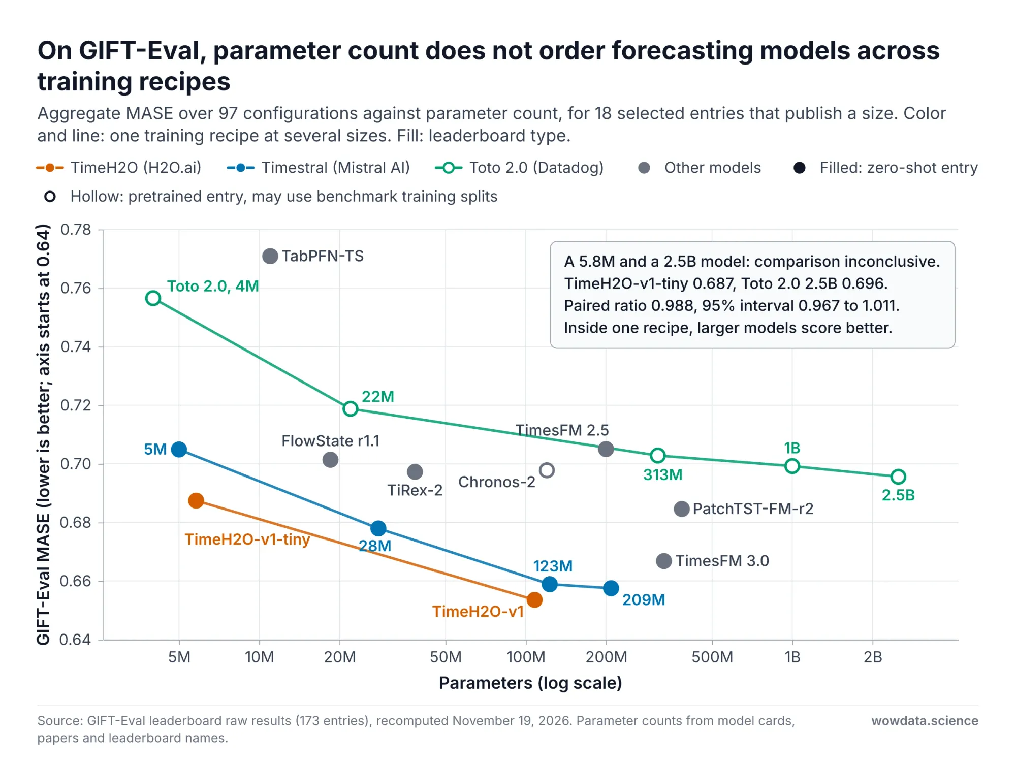
Fig 3: Parameter count against GIFT-Eval error for time series foundation models — wowdata.science
The figure plots the 18 entries of the table that publish a parameter count. Two patterns stand out. Across recipes, size predicts little. The 5.8M-parameter TimeH2O-v1-tiny and the 2.5B-parameter Toto 2.0 cannot be separated (paired MASE ratio 0.988, interval 0.967 to 1.011), and neither can the 5M-parameter Timestral and the 200M-parameter TimesFM 2.5 (ratio 1.000, interval 0.981 to 1.025). Within a recipe, size predicts a lot: Toto 2.0 improves from 0.757 to 0.696 as it grows from 4M to 2.5B, and TimeH2O from 0.687 to 0.654 as it grows from 5.8M to 108M.
A table of means cannot say whether two models differ. For that we compared pairs on the same configurations, resampling whole datasets: 5,000 bootstrap resamples over those 28 dataset names. The roster is fixed by rule: TimeH2O-v1 against every other entry among the eleven best single models, plus three older models discussed in this post.
| TimeH2O-v1 compared with | MASE ratio | 95% interval | CRPS ratio | 95% interval |
|---|---|---|---|---|
| PDM-Nano | 1.026 | 0.983 to 1.084 | 1.017 | 0.970 to 1.074 |
| Morpheus-2.0 | 1.012 | 0.936 to 1.094 | 0.969 | 0.893 to 1.042 |
| PDM-Pico | 0.998 | 0.957 to 1.045 | 0.989 | 0.946 to 1.035 |
| Timestral-209M | 0.994 | 0.966 to 1.019 | 0.988 | 0.955 to 1.015 |
| TurkForecast-FM-Chronos2-LoRA-v1 | 0.993 | 0.883 to 1.122 | 1.041 | 0.893 to 1.259 |
| Timestral-123M | 0.992 | 0.961 to 1.019 | 0.984 | 0.950 to 1.012 |
| t0-gamma | 0.989 | 0.946 to 1.054 | 0.975 | 0.932 to 1.036 |
| Falcon-2.0 | 0.981 | 0.945 to 1.019 | 0.906 | 0.858 to 0.957 |
| Lingjiang2.0 | 0.981 | 0.937 to 1.036 | 0.965 | 0.923 to 1.014 |
| TimesFM-3 | 0.980 | 0.961 to 0.996 | 0.967 | 0.940 to 0.989 |
| Granite-PatchTST-FM-r2 | 0.955 | 0.933 to 0.974 | 0.943 | 0.920 to 0.965 |
| Chronos-2 | 0.937 | 0.912 to 0.961 | 0.908 | 0.873 to 0.940 |
| TimesFM-2.5 | 0.927 | 0.904 to 0.949 | 0.898 | 0.872 to 0.924 |
A ratio below 1 favors TimeH2O-v1. In eight of the first nine rows both intervals include 1. Those comparisons are inconclusive, which is not the same as showing that the models are equal. The exception is Falcon-2.0, which is inconclusive on MASE and behind on CRPS. From TimesFM-3 down, the intervals exclude 1. TimeH2O-v1 is ahead of TimesFM-3 by 2.0 percent in MASE and 3.3 percent in CRPS, and ahead of the two models released in autumn 2025, Chronos-2 and TimesFM-2.5, by 6 to 10 percent.
fev-bench covers 100 tasks, 46 of them with covariates, and ships its own bootstrap code. We ran fev 0.10.0 on the results repository at commit 844509e (November 17, 2026), using the scaled quantile loss. The roster is again fixed by rule: every visible entry ranked above TimeH2O-v1 by win rate or skill score, the two ranked directly below it, and the models discussed in this post. Its two summary numbers are the win rate (the share of tasks on which one model has the lower loss) and the skill score, which the pairwise table reports as error reduction: one minus the geometric mean ratio of the two models' losses.
| TimeH2O-v1 compared with | Win rate | 95% interval | Error reduction | 95% interval |
|---|---|---|---|---|
| TimeRSI-1.5 (closed API) | 43% | 33 to 52 | -2.1% | -3.5 to -0.7 |
| ci-proto | 50% | 40 to 59 | -1.4% | -3.1 to 0.1 |
| TimeRSI (closed API) | 55% | 45 to 65 | -0.8% | -2.7 to 1.0 |
| Timestral-209M | 54% | 43 to 63 | 0.9% | -0.1 to 1.9 |
| PDM-Nano (closed API) | 59% | 49 to 68 | 1.0% | -0.2 to 2.2 |
| t0-gamma | 67% | 58 to 76 | 2.8% | 1.5 to 4.2 |
| TimesFM-3 | 77% | 69 to 85 | 3.6% | 2.2 to 5.0 |
| Chronos-2 | 88% | 82 to 94 | 6.7% | 5.1 to 8.5 |
| TabPFN-TS-3 | 91% | 85 to 96 | 13.5% | 10.8 to 16.3 |
| TimesFM-2.5 | 93% | 88 to 98 | 14.9% | 11.7 to 18.4 |
| Seasonal naive | 100% | 100 to 100 | 50.8% | 46.2 to 55.4 |
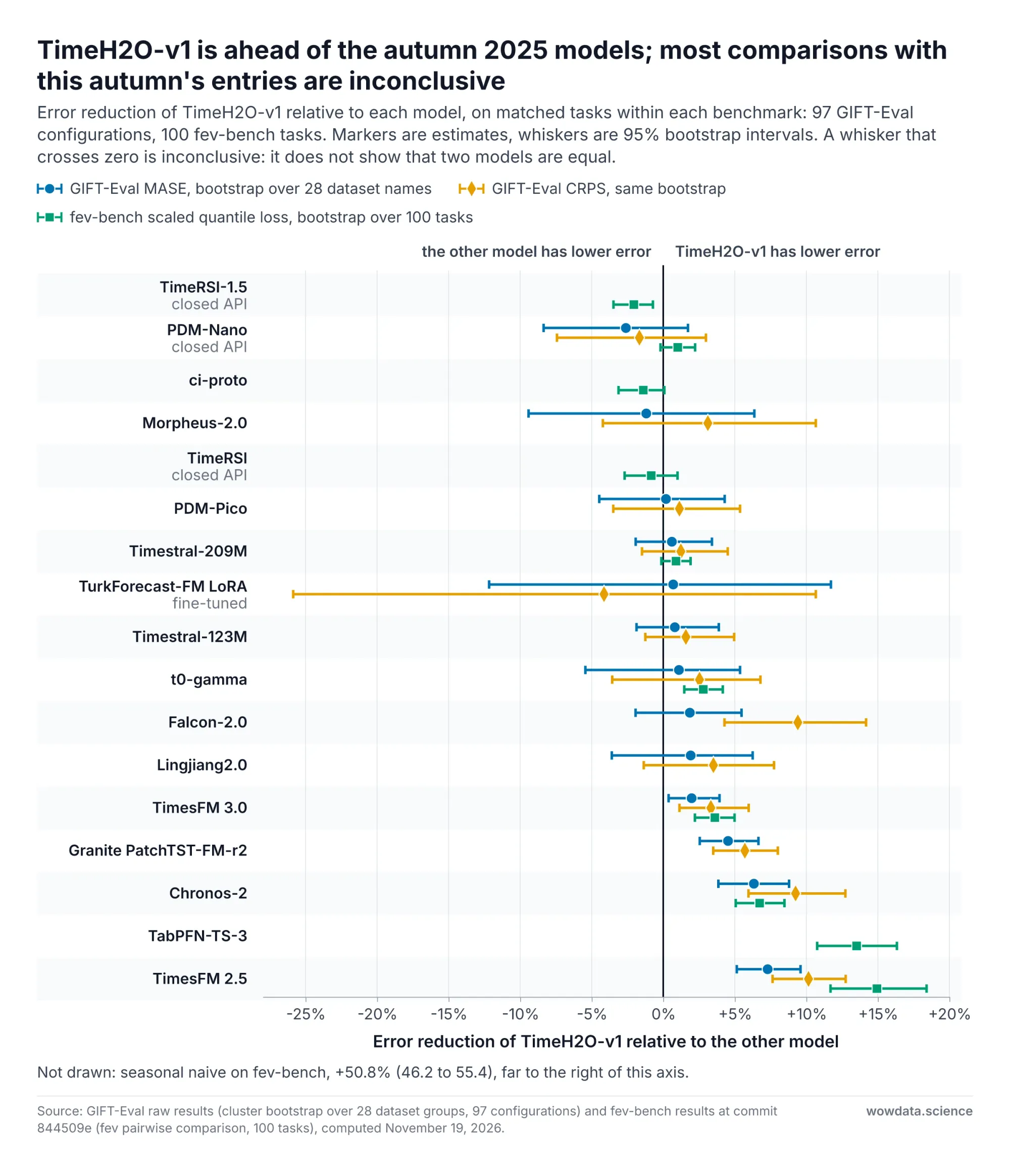
Fig 4: Paired comparisons of TimeH2O-v1 with other forecasters on GIFT-Eval and fev-bench — wowdata.science
The 50.8 percent skill score against the seasonal naive baseline matches the figure H2O read from the leaderboard on October 24, when it reported the model first of 32. The repository's results on November 17 hold 40 visible entries, and the picture around TimeH2O-v1 is different. TimeRSI-1.5 is ahead of it with an interval that excludes zero. That entry is a closed API that the benchmark's metadata does not class as zero-shot. Its results were committed on October 23, a day before H2O read the board, so new entries alone do not explain the difference between the two readings. H2O says its ranking is "with non-commercial models included". It does not say whether closed APIs were included. ci-proto, added on November 11, has the higher point estimate, with an interval that includes zero. The comparisons with the older TimeRSI entry, Timestral-209M and PDM-Nano are also inconclusive.
PDM-Nano is a reminder that a ranking depends on the benchmark. Its point estimate is ahead of TimeH2O-v1 on GIFT-Eval and behind it on fev-bench, and neither interval excludes zero.
The summary for a practitioner: on fev-bench the leading models roughly halve the scaled quantile loss of a seasonal naive forecast, and on GIFT-Eval they cut its MASE by about a third. Among the eleven best single models, MASE spans 0.637 to 0.667, and eight of TimeH2O-v1's ten paired comparisons on that set are inconclusive. CRPS can differ more: TimeH2O-v1 is about 9 percent ahead of Falcon-2.0 on it. Against Chronos-2 and TimesFM-2.5, both released in autumn 2025, TimeH2O-v1 is 6 to 15 percent ahead.
Tabular Foundation Models on TabArena and TALENT
We could not recompute the tabular boards in the same way, so the numbers below are vendor-reported. They come from the Mitra-v2 technical report, which evaluates on TabArena under its one-hour protocol and on TALENT. Both boards rank methods by Elo, a rating computed from pairwise wins across datasets.
| Board (Elo) | Mitra-v2 | TabFM | EXAONE Tabular | TabPFN-3 | TabICLv2 |
|---|---|---|---|---|---|
| TabArena overall, 51 datasets | 1,775 | 1,774 | 1,749 | 1,638 | 1,568 |
| TabArena binary, 30 datasets | 1,754 | 1,791 | 1,748 | 1,654 | 1,587 |
| TabArena multiclass, 8 datasets | 1,810 | 1,690 | 1,809 | 1,581 | 1,547 |
| TabArena regression, 13 datasets | 1,986 | 1,987 | 1,880 | 1,798 | 1,682 |
| TALENT overall, 274 datasets | 1,480 | 1,503 | 1,452 | 1,415 | 1,400 |
Source: Amazon's Mitra-v2 technical report. We did not rerun these evaluations. Elo values are not comparable across boards. Amazon's own reading is careful: the report calls the top of the overall and classification boards a "statistical tie", and notes that the regression board rests on 13 datasets with wide intervals. Against its predecessor the picture is clearer: Amazon's article says Mitra-v2 produces a better result than Mitra-v1 on 32 of the 33 datasets where both run natively.
Three cautions apply before anyone quotes a winner.
- Vendors report first-place results under different evaluation rules. The TabPFN-3 report (May) says a forward pass of TabPFN-3 outperforms all other models on TabArena. The EXAONE Tabular report (August 26) says its classification model ranks first overall. Mitra-v2 (September 3) reports the highest overall point estimate. The TabFM paper (September 29) says zero-shot TabFM ranks first among default tabular foundation models. The protocols differ in fine-tuning, bagging, time budget and what counts as a default.
- The splits are random. TabArena uses repeated cross-validation. TabReD showed on eight industry datasets with timestamps that time-based splits produce a different ranking of methods than random splits do.
- Even basic facts conflict. The Mitra-v2 and EXAONE reports describe TabFM as a 1.6B-parameter model. Google's later paper describes a 400M-parameter checkpoint. We could not determine whether these refer to the same weights.
The Hypothesis: Context Policy Versus Model Choice
Here is the hypothesis this research plan is built to test. It is stated so that it can fail.
On time-ordered data, and within ranges a real deployment would use, changing the context policy at a fixed model changes error at least as much as swapping the model at a fixed policy.
A context policy, as defined at the top, is the rule that decides what the model sees at inference: which rows or how much history, how many, how fresh, and which covariates. In this post "context" always means that input. "Support set" is the tabular name for it, and "history" the forecasting name.
The two lists below draw on different studies with different protocols. They illustrate orders of magnitude. They cannot be compared directly with each other.
Evidence that motivates the hypothesis
- The Mitra-v2 report swept the prediction-time support cap from 512 to 32,768 rows on the six largest classification and six largest regression tables of TabArena, with everything else fixed, on one split per dataset with the fine-tuned recipe. Error fell by 28 percent for classification and 21 percent for regression in geometric mean.
- In the same report, raising only that cap from 8,192 to 32,768 rows moved the regression rating from 1,848.4 to 1,935.9 Elo. For scale, the whole gap between Mitra-v2 and EXAONE Tabular on that board is about 106 Elo. The report concludes that "the same released weights can be moved by tens of Elo purely through deployment configuration".
- The same report finds that on TALENT, adding validation rows to the context moved EXAONE Tabular by 67 Elo, TabFM by 25 and Mitra-v2 by 11.
- Covariates are part of the context. The t0 report passes known-future covariates to one fixed checkpoint on 30 fev-bench tasks, and its skill score rises from 36.7 to 43.0, a gain of 6.3 points (95% interval 2.2 to 10.9). That corresponds to about 10 percent lower error on those tasks. The gain is not universal: 19 of the 30 tasks improved and 11 got worse.
- Short contexts are expensive on high-frequency data. In the same report, on a 12-pair subset of GIFT-Eval, capping the history at 64 points costs hourly series 42 percent in CRPS and daily or slower series 3.7 percent.
Evidence against it
- The gain from more rows saturates. In the Mitra-v2 sweep, a cap of 8,192 rows already realizes 94 percent of the total error reduction for classification and 92 percent for regression.
- The same report tried to choose support rows more cleverly and reports that "picking the support rows by stratified or clustering-based selection did not help and sometimes hurt". Raising the classification support cap well past its released value reduced accuracy.
- The large ablation effects concern how many rows, not which rows, and they were measured on random splits.
- Beyond a moderate length, more history buys little. On its 12-pair GIFT-Eval subset, the t0 report finds CRPS within 5 percent of the value at the full 8,192-point cap from a 1,024-point cap, and within 1 percent from 4,096. Many of those series are short: the realized context at the full cap averages about 1,000 points. In the report's hourly electricity backtest, going from 512 to 8,192 hours of history changed each model's error by between +2 and -15 percent, while the models differed from each other by more than that at either length.
- Model-side work pays. With the backbone unchanged, a new prior and optimizer took Mitra from v1 to v2, which Amazon's article reports as better on 32 of 33 datasets. O'Prior holds architecture, optimizer and compute budget fixed and reports that the synthetic prior alone changes accuracy substantially.
- Scale pays within a recipe, as the Toto 2.0 rows above show.
- Drift can be handled inside the model. Drift-Resilient TabPFN pretrains on structural causal models that shift over time and reports accuracy rising from 0.688 to 0.744 across 18 datasets.
- If time-based splits reshuffle rankings, as TabReD found, model choice may matter more on time-ordered data than random-split leaderboards suggest.
Read together, the published evidence says that short contexts can be costly and that the gain from more context flattens. Whether model swaps then matter more is an open question. We did not find a study that measures both effects on the same time-ordered data with the same protocol. That is the gap the plan addresses. The pilot in the next section is a first look, on one dataset.
There is also a practical reason to ask the question. Serving routes range from a 512-point default in one managed function to a 15,360-point maximum for self-hosted weights. That is a motivation, not evidence about the answer.
One more condition makes the comparison fair. A deployment can serve a poor context policy, and it can also serve last year's model. If the policy side may include bad choices while the model side is limited to a handful of leaders within 5 percent of each other, the hypothesis wins by construction. The plan therefore fixes both ranges in advance and in the same way: policy levels that a team might choose deliberately, and model levels that include at least one model a year old as well as current leaders. The comparison is reported for the narrow model range and for the wide one. On tables the model contrast is Mitra-v1 against Mitra-v2, which share an architecture. A second model family counts as confirmatory only if it is named before any test origin is opened.
Pilot Results for Tabular and Time Series Foundation Models
To check that the design is workable we ran a small pilot on one NVIDIA A10G. It uses a single public dataset, OpenML 151 "electricity": 45,312 half-hourly rows from the New South Wales electricity market, from May 1996 to December 1998, in time order. Each row has the day of the week, the period of the day, the price and demand in New South Wales, the price and demand in Victoria, and the scheduled transfer between the two states. The label says whether the New South Wales price is above or below its average over the previous 24 hours. The demand series has no gaps.
The pilots use rolling origins. An origin is a cut point in time: rows before it may be used as context, and rows after it are predicted. Rolling means the cut is repeated at several points along the series.
Read these numbers as a feasibility check. One dataset cannot support a general claim, and the last two subsections say what the pilot does and does not show.
Pilot 1: Which Rows Go into the Context
Setup. Eight rolling origins across the second half of the stream. At each origin the model classifies the next 1,000 rows, about three weeks, from a context of 512, 2,048 or 8,192 rows drawn from before the origin. Three policies choose those rows: the most recent rows, a uniform random sample of all history, and a mix of half each. The models are the Mitra-v2 classifier and the Mitra-v1 classifier, both zero-shot, and LightGBM trained on exactly the same rows.
What is known when. This is not a forecast. Each row arrives with its own measurements, and the model must say whether its price is above the recent average without being given that average. Only the labels are delayed: no label from the three-week block is used. Pilot 1b shortens that delay to one day.
import numpy as np

def context_index(policy, t, n, seed):
    """Row indices for a context of n rows, using only rows before origin t."""
    rng = np.random.default_rng(seed)
    if policy == "recent":
        return np.arange(t - n, t)
    if policy == "uniform":
        return np.sort(rng.choice(t, size=n, replace=False))
    if policy == "mixed":
        half = n // 2
        old = rng.choice(t - half, size=n - half, replace=False)
        return np.sort(np.concatenate([old, np.arange(t - half, t)]))
    raise ValueError(policy)
Repeatability. Because zero-shot Mitra predictions change from call to call, we ran every configuration three times with different seeds, and the two sampled policies with three different row samples each. All numbers are averages. A single call moved by up to 0.10 between runs, but the averages are stable: across the three runs, a paired difference moved by 0.006 on average and by 0.030 at most. LightGBM was identical in every run. What limits this pilot is the variation between its eight origins, not the noise between runs.
Statistics. Differences are paired by origin. In these comparisons a percentile bootstrap over eight origins gave narrower intervals than a t interval, so we report the wider 95 percent t interval and the p-value of a sign-flip permutation test. Both rest on assumptions that eight blocks of one stream do not guarantee: that the eight differences are independent, and, for the test, that each is as likely to fall on either side of zero when there is no effect. The intervals and p-values are therefore nominal. The analysis computes about 90 paired comparisons for Pilot 1 and Pilot 1b, and nothing is adjusted for that. With eight origins the smallest attainable p-value is about 0.008, so no single comparison could survive such an adjustment. Everything in Pilot 1 and Pilot 1b is exploratory, and an interval that narrowly excludes zero should not be read as a finding.
Result with the cutoff at the origin. Mean log-loss over eight origins, lower is better. Always predicting the base rate of the context scores 0.68, and LightGBM trained on all history scores 0.591.
| Context rows | Policy | Mitra-v2 | Mitra-v1 | LightGBM on the same rows |
|---|---|---|---|---|
| 512 | Recent | 0.792 | 0.834 | 1.793 |
| 512 | Uniform | 0.580 | 0.590 | 0.916 |
| 512 | Mixed | 0.597 | 0.590 | 1.050 |
| 2,048 | Recent | 0.553 | 0.524 | 0.848 |
| 2,048 | Uniform | 0.555 | 0.562 | 0.792 |
| 2,048 | Mixed | 0.548 | 0.522 | 0.745 |
| 8,192 | Recent | 0.554 | 0.542 | 0.628 |
| 8,192 | Uniform | 0.547 | 0.558 | 0.645 |
| 8,192 | Mixed | 0.523 | 0.525 | 0.613 |
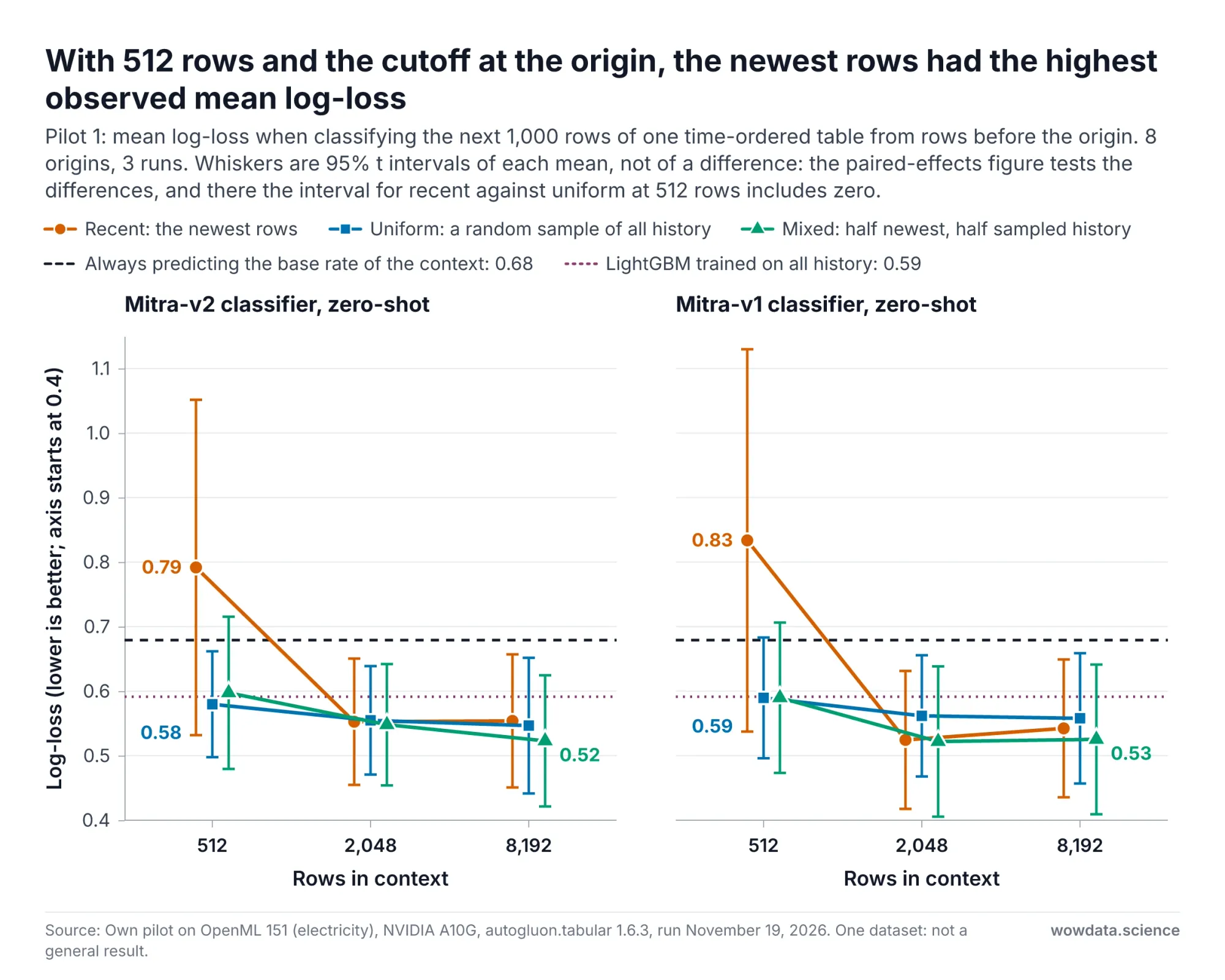
Fig 5: Pilot 1 log-loss of Mitra-v2 and Mitra-v1 by context policy and size on one electricity dataset — wowdata.science
Four observations for Mitra-v2:
- With 512 rows, the newest rows alone had the highest error. The recent policy was worse than the uniform one by 0.212 log-loss and was better at only one of eight origins. The t interval runs from -0.037 to 0.461 and the sign-flip p-value is 0.06: suggestive, not conclusive. Its mean of 0.79 was also above the 0.68 of always predicting the base rate, a comparison that is inconclusive too. The policy beat the base rate at five origins and was far worse at three.
- At larger context sizes the two simple policies could not be separated. Recent minus uniform was -0.002 at 2,048 rows (interval -0.065 to 0.061) and 0.007 at 8,192 (interval -0.031 to 0.045).
- The mixed policy had the lowest observed mean at 8,192 rows, without a clear difference. Mixed minus uniform was -0.024 (interval -0.063 to 0.015, better at five of eight origins). The three runs agreed on it (-0.026, -0.026, -0.019). The eight origins do not.
- Swapping the checkpoint changed little. Mitra-v2 minus Mitra-v1 ranged from -0.042 to 0.028 across the nine cells, and every t interval includes zero. The largest difference, for 512 recent rows, has a sign-flip p-value of 0.03. Contexts of 2,048 and 8,192 rows are also longer than the 512 support rows Mitra-v1 was pretrained on, so those cells mix the checkpoint with extrapolation. Mitra-v2 beat LightGBM on the same rows in every cell, with intervals that exclude zero.
A dataset artifact, and a check. In this dataset the three Victoria columns are constant for the first 17,424 rows. A uniform sample of all history therefore mixes two feature regimes, while the test blocks and the recent rows lie in the later one. We repeated the 512-row and 2,048-row cells with history sampled only from rows after that point. The direction and size of the difference were similar: with 512 rows the uniform sample scored 0.550 and the recent rows 0.793, a difference of 0.243 (interval 0.001 to 0.485, p = 0.02), and it stays exploratory. With 2,048 rows the difference was 0.014, with an interval that includes zero.
The recent contexts were closer to the query rows in feature space. The drift score, the AUC of a classifier trained to tell context rows from query rows, was 0.55 for 512 recent rows, where 0.5 means this classifier does no better than chance. For a uniform sample it was 0.83, or 0.78 once the constant-column rows are excluded. Being close in features did not help. One possible explanation is that a narrow recent window covers too few market conditions for the three weeks that follow. The pilot did not test that explanation, but it suggests looking at how old the cutoff is.
Pilot 1b: How Fresh the Context Is
Setup. Each 1,000-row block is scored in chunks of 48 rows, one day. For every chunk the context is drawn twice, with the same size, the same sampling seed and the same model random stream. One arm keeps its cutoff at the block origin: it draws only from rows before the origin, so labels are up to three weeks late. The other arm advances its cutoff daily: it draws from rows before the chunk, so labels are at most a day late. On the first day the two arms see the same context and must give identical predictions, and they did: the largest difference in predicted probability was zero. Both arms build a context for every daily chunk, on the same schedule. One builds it from a fixed eligible history and the other from a growing one, and that cutoff is the only thing that differs in the rule. For the recent policy the two contexts then differ only by their newer rows. For the two sampled policies both arms resample for each chunk, and only the daily-cutoff arm samples from a growing pool. Neither arm reuses one fixed set of rows for three weeks. Pilot 1 above does that. Context sizes of 512 and 2,048 rows, two runs.
The replay below plays back the recorded scores of the experiment for one cell: the newest-rows policy with a 512-row context, the first row of the table that follows. It is the cell with the largest change of the six in that table, so it shows the effect at its strongest. After a setup frame, each frame is one day, and the last frame adds the 21-day result. The top card shows the stream and the rows each arm reads from it. With the cutoff left at the origin, the arm keeps the 512 rows that end there, and the newer rows it does not use pile up day after day. With a daily cutoff, the arm takes the newest 512 rows before each day. The middle card shows that day's log-loss at each of the eight origins, one row per origin with the two arms joined, and the chart below it draws the mean of the eight. The model is the same in both arms: only the rows it is given differ. A log-loss above the natural logarithm of 2, about 0.693, is worse than answering 50/50 on every row. The figure uses this fixed reference because it does not depend on the context. The 0.68 quoted above is the log-loss of always predicting the base rate of the context. The log-loss values are recorded scores, the strips and row counts follow from the rule of each arm, and no scores are computed between two days. The first frame shows the final state.
The replay shows when the origin cutoff falls behind. It does not show why, and it says nothing about the other policies. A uniform sample with its cutoff left at the origin scored 0.579 on the same blocks, against 0.599 for the newest rows with a daily cutoff, a difference we did not test.
Fig 6: Pilot 1b replayed day by day with the context cutoff left at the origin or advanced daily (animated) — wowdata.science
Mean log-loss of the zero-shot Mitra-v2 classifier over eight origins:
| Context rows | Policy | Cutoff at the origin | Cutoff advanced daily | Change | 95% t interval | Sign-flip p | Origins where daily was better |
|---|---|---|---|---|---|---|---|
| 512 | Recent | 0.788 | 0.599 | -0.188 | -0.362 to -0.015 | 0.03 | 7 of 8 |
| 512 | Uniform | 0.579 | 0.570 | -0.009 | -0.027 to 0.010 | 0.30 | 6 of 8 |
| 512 | Mixed | 0.576 | 0.494 | -0.083 | -0.174 to 0.009 | 0.09 | 6 of 8 |
| 2,048 | Recent | 0.547 | 0.516 | -0.031 | -0.066 to 0.005 | 0.08 | 7 of 8 |
| 2,048 | Uniform | 0.561 | 0.540 | -0.021 | -0.052 to 0.010 | 0.19 | 6 of 8 |
| 2,048 | Mixed | 0.547 | 0.507 | -0.040 | -0.081 to 0.000 | 0.05 | 6 of 8 |
The origin-cutoff column was measured again in one-day chunks, and the two sampled policies drew a new row sample for every chunk, so it differs slightly from the table in Pilot 1.
- Freshness helped the newest-rows context most. With 512 rows, a daily cutoff improved the recent policy by 0.188, with an interval that excludes zero. The mixed policy improved by 0.083, with an interval that just includes zero.
- At 2,048 rows the gains were small. They were 0.031 for the recent policy and 0.040 for the mixed one, each better at six or seven of eight origins, with intervals that include or touch zero.
- A uniform sample barely moved. The changes were 0.009 and 0.021. One more day changes little in a sample drawn from months.
- With a daily cutoff, mixed was ahead of uniform at the small context size, an exploratory result. The difference was 0.076 at 512 rows (interval 0.009 to 0.144, p = 0.02, seven of eight origins). At 2,048 rows it was 0.033, with an interval that includes zero.
- Recent rows alone were no better than a uniform sample even when fresh. At 512 rows the recent policy was 0.029 worse, with an interval from -0.086 to 0.144.
- The origin-cutoff arm was worse in each of the three weeks, most in the second. With the newest 512 rows and the cutoff at the origin, the log-loss was 0.65 over days 1 to 7, 0.93 over days 8 to 14 and 0.78 over days 15 to 21. With a daily cutoff it was 0.53, 0.63 and 0.64. The ranking varies by day. The daily cutoff had the lower mean on 15 of the 21 days and the higher one on days 4, 10, 12, 15 and 19, with day 1 identical by construction. The largest single-day gap was on day 8, 1.38 against 0.40, and a single day is a mean of eight origins with a wide spread.
The lowest mean log-loss we observed in the pilot was 0.494, for 512 rows, mixed, with a daily cutoff. We did not test whether it differs from the larger contexts with an origin cutoff, such as 0.523 for 8,192 mixed rows.
LightGBM trained on the same rows moved in the same direction, from a mean of 1.79 to 1.24 for the newest 512 rows, with an interval that includes zero. The effect does not look specific to in-context learning. One caution on what "daily" assumes: labels must arrive within a day. Here the label can be computed as soon as prices are published. Many operational labels arrive much later.
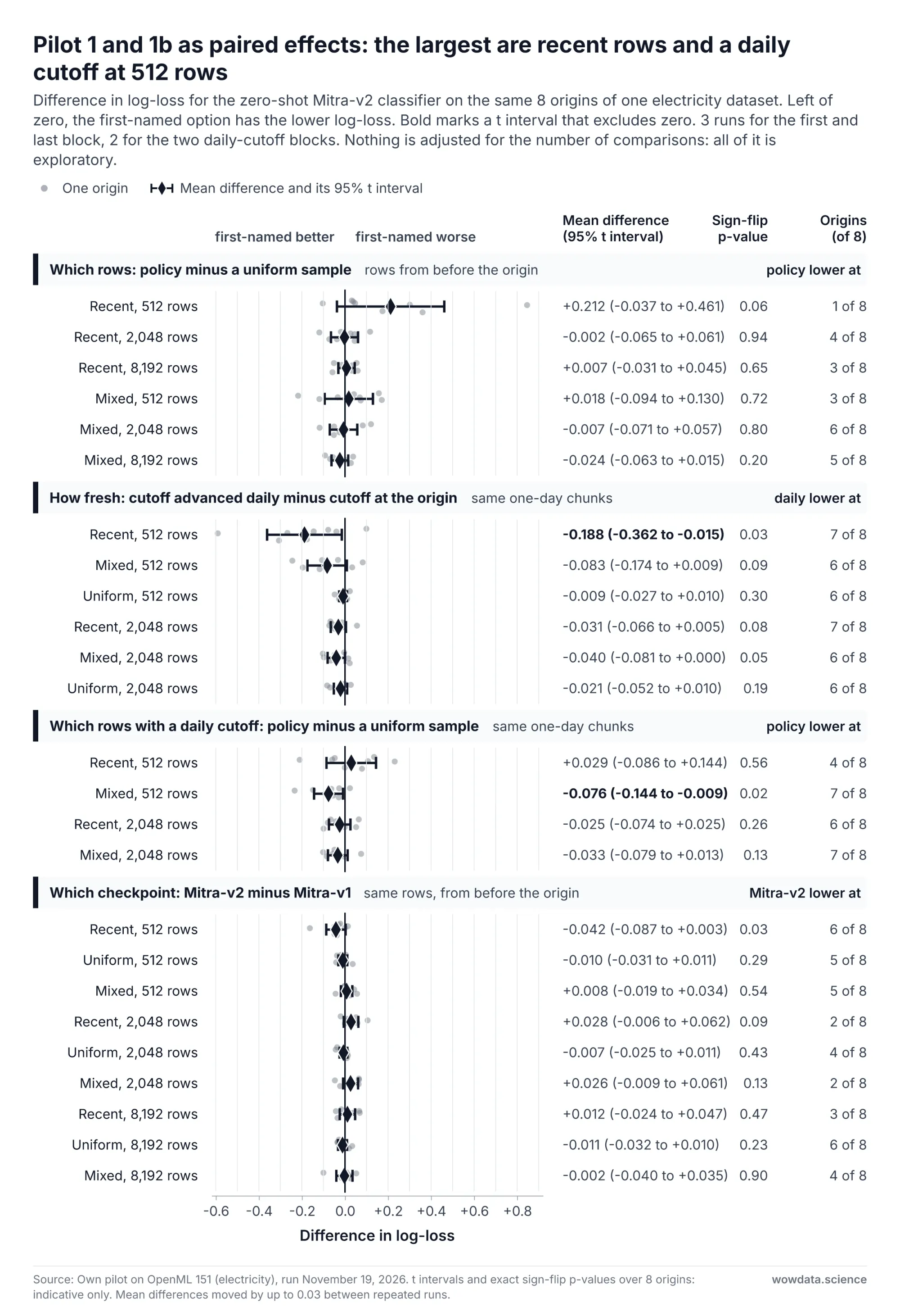
Fig 7: Pilot 1 and 1b paired log-loss differences for row selection and context cutoff and checkpoint on one electricity dataset — wowdata.science
One caution on the checkpoint comparison. Amazon reports Mitra-v2 ahead of Mitra-v1 on 32 of 33 TabArena datasets with its fine-tuned recipe. Our comparison is zero-shot on one drifting dataset, so the absence of a clear difference here says more about this setup than about the two models.
Pilot 2: Context Length for TimesFM 2.5 and Chronos-2
Setup. The half-hourly demand series from the same dataset. 45 rolling origins, ten days apart. Horizon 96 steps, two days. TimesFM 2.5 and Chronos-2, both zero-shot and univariate, each given the most recent 128, 512, 2,048 or 8,192 points.
Metrics. MASE is the mean absolute error of the median forecast over the horizon, divided by the mean absolute error of a daily seasonal naive forecast over all observations before the origin. That denominator is the same for every model and history length at an origin. WQL (weighted quantile loss) is the average across origins of a per-origin score. At each origin, twice the summed pinball loss is divided by the summed absolute target, and that ratio is averaged over the nine quantile levels. Coverage is the share of actual values inside the 10 to 90 percent interval.
import torch
from chronos import Chronos2Pipeline

pipe = Chronos2Pipeline.from_pretrained("amazon/chronos-2", device_map="cuda")
levels = [0.1, 0.2, 0.3, 0.4, 0.5, 0.6, 0.7, 0.8, 0.9]
quantiles, mean = pipe.predict_quantiles(
    [torch.tensor(history[-2048:])], prediction_length=96, quantile_levels=levels)
q = quantiles[0].reshape(96, 9)                # one series, 96 steps, 9 quantiles
The replay below is one origin, forecast again and again as the history grows from 96 to 8,192 points. Every frame is a real model output, and the line under the charts names the phase the replay is in. We picked the origin by a fixed rule, to illustrate the mean result. Of the 14 origins where the better model matched the 45-origin mean at all four tested lengths, it is the one closest to that mean. That only 14 of 45 origins qualify is a reminder that a single forecast window is noisy.
Fig 8: Pilot 2 replay at one origin selected to match the aggregate ranking (animated) — wowdata.science
| History | TimesFM 2.5 MASE | Chronos-2 MASE | TimesFM 2.5 WQL | Chronos-2 WQL | TimesFM 2.5 coverage | Chronos-2 coverage |
|---|---|---|---|---|---|---|
| 128 points, 2.7 days | 0.803 | 1.469 | 0.090 | 0.181 | 84% | 60% |
| 512 points, 10.7 days | 0.562 | 0.840 | 0.064 | 0.099 | 83% | 65% |
| 2,048 points, 42.7 days | 0.583 | 0.490 | 0.068 | 0.057 | 69% | 75% |
| 8,192 points, 170.7 days | 0.556 | 0.477 | 0.064 | 0.055 | 74% | 79% |
For reference, the weekly seasonal naive forecast scores a MASE of 0.779 and the daily one 1.267.
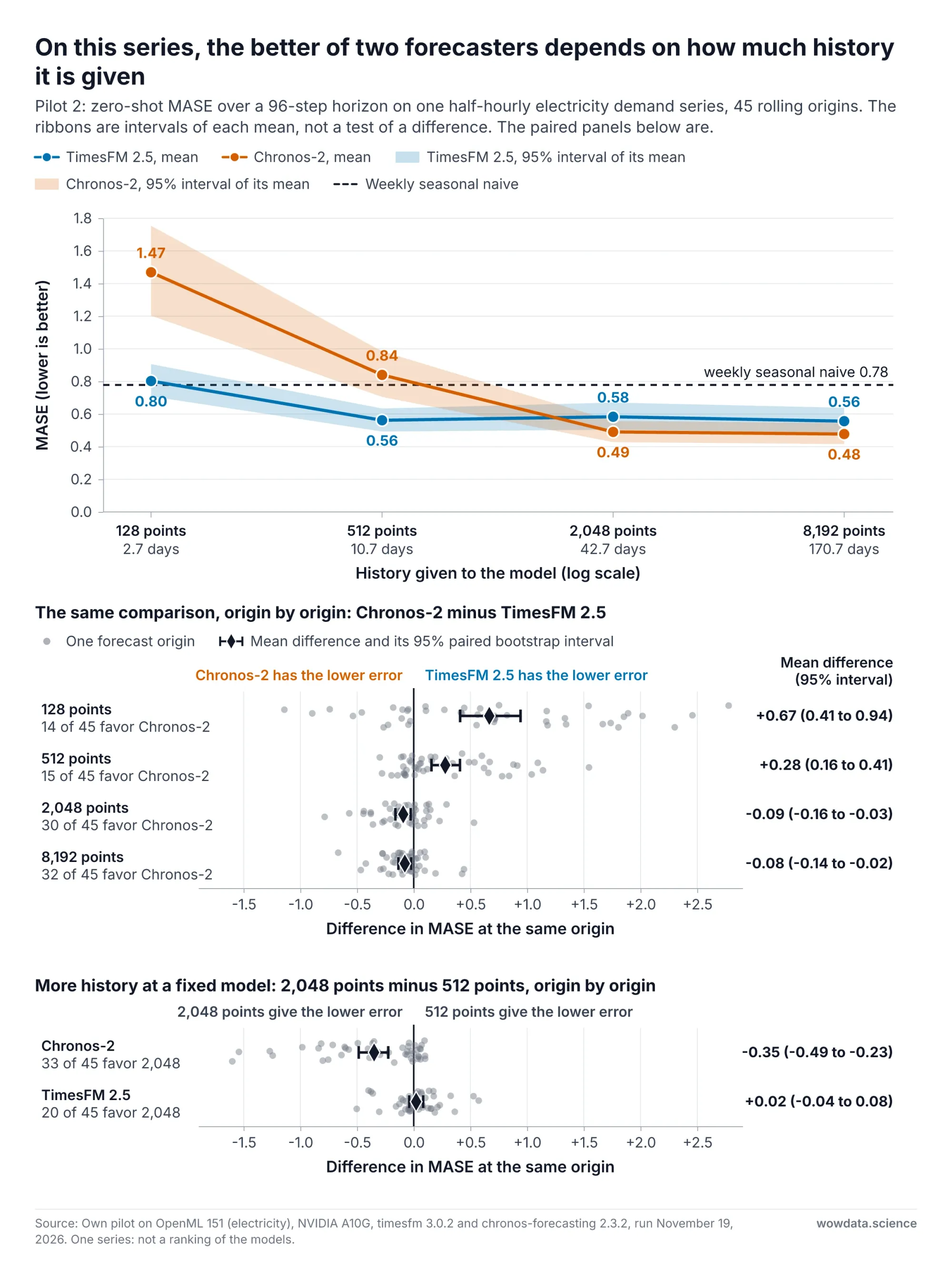
Fig 9: Pilot 2 forecast error and paired differences by history length on one electricity series — wowdata.science
Differences are paired by origin, with a percentile bootstrap interval over the 45 origins. The origins are ten days apart on one series and are not independent, so we also computed a moving-block bootstrap with blocks of five consecutive origins. It gave similar intervals, quoted where they matter.
- History length mattered for one model. For the other the result was inconclusive. Going from 512 to 2,048 points lowered Chronos-2's MASE by 0.350 (interval 0.225 to 0.485, better at 33 of 45 origins). The same change moved TimesFM 2.5 by 0.021 in the other direction, with an interval from -0.040 to 0.083. From 2,048 to 8,192 points neither model changed clearly.
- The ranking reversed. At 512 points TimesFM 2.5 was ahead by 0.278 (interval 0.156 to 0.408). At 2,048 points Chronos-2 was ahead by 0.093 (interval 0.027 to 0.162, block bootstrap 0.047 to 0.145), and at 8,192 points by 0.079 (interval 0.023 to 0.135). Chronos-2 had the lower error at 15 of 45 origins with 512 points and at 30 of 45 with 2,048.
- With 512 points, Chronos-2 could not be separated from a naive baseline. Its difference from the weekly seasonal naive forecast was 0.061, with an interval from -0.082 to 0.208.
- Calibration moved too. Coverage of the nominal 80 percent interval ranged from 60 to 79 percent for Chronos-2 and from 69 to 84 percent for TimesFM 2.5.
On this series the answer to "which model is better" was "it depends on how much history you pass". A leaderboard cannot tell you that, because its entries are not a crossed comparison at the same history lengths.
We do not know why Chronos-2 does so much better with more than 512 points here. Chronos-2 forecast the origins in batches of up to 16, so we checked whether batching plays a part. At the origin shown in Fig 8, forecasting it alone reproduced the batched Chronos-2 MASE to six decimal places at the four history lengths in the table (128, 512, 2,048 and 8,192). At that origin the Chronos-2 error dropped between 512 and 768 points, and 768 is the first length we tried that covers more than two weeks. That is one origin, and the two-week explanation is a guess.
Pilot 3: A Tabular Model as a Forecaster
Setup. The same series, horizon and metrics as Pilot 2, on four of its origins, because every Mitra-v2 regression fit is a full bagged fine-tune of about five minutes. Forecasting is recast as tabular regression. Each row is one half-hour, with nine features: period of day, day of week, the demand 96, 144, 192, 336 and 672 steps earlier, and the means of one earlier day and one earlier week. Every feature is at least 96 steps older than its target, so one feature set serves the whole horizon. The cost is that the first forecast step sees nothing from the two days before the origin, while the last step reads the latest observation. The training table has 2,000 rows, chosen as the newest rows or as a uniform sample of history. Those rows are used for fine-tuning as well as for context, so this is training-row selection rather than a pure context policy. The table and the figure report one run, and the random state of the Mitra-v2 fine-tune was not controlled.
| Model | Input | MASE | WQL | Coverage of the 80% interval |
|---|---|---|---|---|
| Mitra-v2 regressor | Newest 2,000 rows | 0.525 | 0.063 | 79% |
| Mitra-v2 regressor | 2,000 sampled rows | 0.632 | 0.073 | 68% |
| LightGBM quantile regression | Newest 2,000 rows | 0.541 | 0.069 | 42% |
| LightGBM quantile regression | 2,000 sampled rows | 0.549 | 0.063 | 65% |
| TimesFM 2.5 | Last 512 points | 0.526 | 0.062 | 90% |
| TimesFM 2.5 | Last 2,048 points | 0.659 | 0.074 | 66% |
| TimesFM 2.5 | Last 8,192 points | 0.460 | 0.054 | 79% |
| Chronos-2 | Last 512 points | 1.070 | 0.136 | 58% |
| Chronos-2 | Last 2,048 points | 0.394 | 0.046 | 78% |
| Chronos-2 | Last 8,192 points | 0.413 | 0.048 | 81% |
| Weekly seasonal naive | Not applicable | 0.550 | Not applicable | Not applicable |
| Daily seasonal naive | Not applicable | 1.309 | Not applicable | Not applicable |
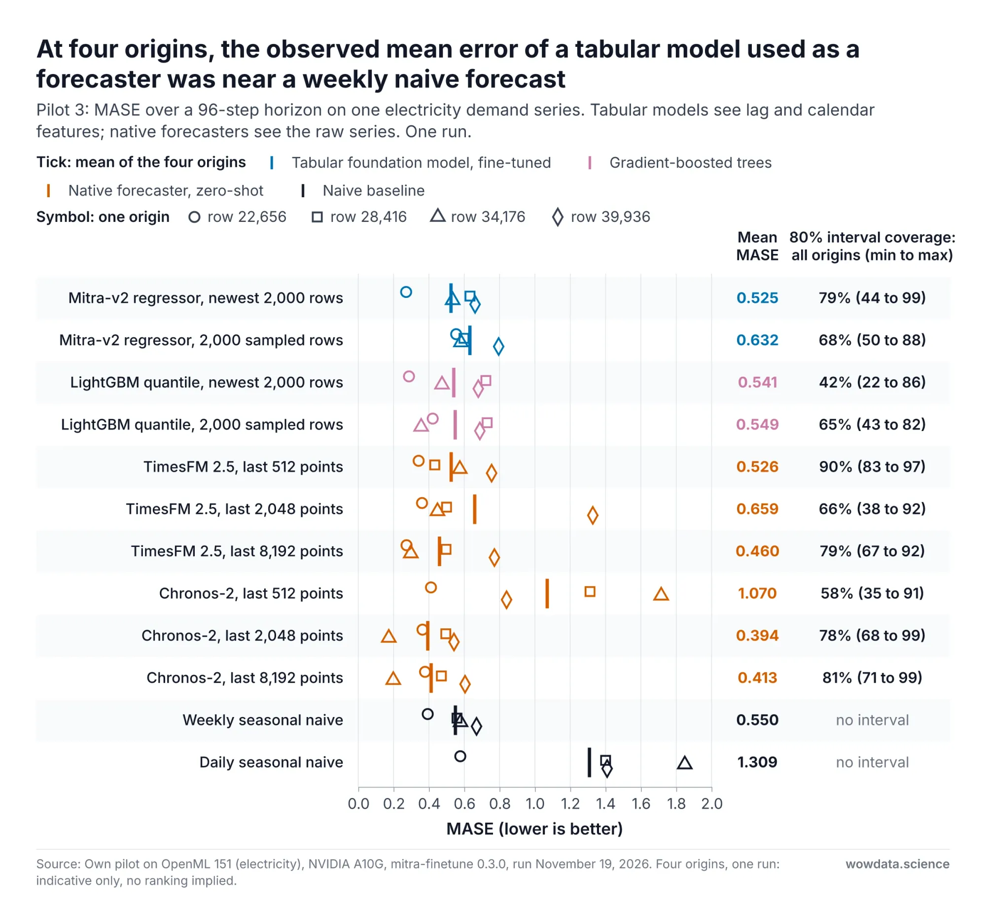
Fig 10: Pilot 3 Mitra-v2 regressor as a forecaster at four origins — wowdata.science
Four origins support observations, not a ranking. How noisy four origins are shows in the TimesFM 2.5 rows, where the mean goes from 0.53 to 0.66 to 0.46 as the history grows.
- The tabular route was workable. The Mitra-v2 regressor on the newest rows had a mean MASE of 0.525, close to LightGBM on the same features (0.541) and to the weekly seasonal naive forecast (0.550).
- Native forecasters landed both below and above the tabular means. Chronos-2 scored 0.39 with 2,048 points and 1.07 with 512.
- With the newest rows, Mitra-v2 had higher interval coverage than LightGBM overall, and its coverage varied by origin. Across the four origins combined, Mitra-v2's 80 percent interval covered 79 percent of the actual values, against 42 percent for LightGBM quantile regression on the same rows. At single origins the Mitra-v2 coverage ranged from 44 to 99 percent.
- Newest rows had the lower error at three of four origins. For Mitra-v2 they gave a lower error than sampled rows at three origins and a higher one at the fourth. Four origins cannot tell that apart from chance.
A second run. On November 20 we ran the Mitra-v2 and LightGBM rows of the table again, at the same four origins. The seeded LightGBM scores were identical. The Mitra-v2 regressor had a mean MASE of 0.511 on the newest rows and 0.635 on sampled rows, where the table has 0.525 and 0.632. Its coverage on the newest rows, across the four origins combined, was 77 percent in place of 79. The newest rows again had the lower error at the same three origins.
What the Pilot Says About the Hypothesis
The hypothesis compares a change of context policy with a swap of the model. The pilot cannot test that. It has one dataset, no current leader among its forecasters, and a tabular swap between two checkpoints of one family.
What it shows is narrower.
- The largest observed effects came from short contexts. Changing which 512 rows a tabular model sees, advancing the cutoff of a 512-row context of recent rows, and extending a forecaster's history from 512 to 2,048 points each moved the mean error by roughly 0.2 log-loss or 0.35 MASE. Only the last of these is clear on this series, and its block-bootstrap check gave similar intervals.
- With more context, the observed effects were small. From 2,048 rows, Mitra-v2's row-selection policies could not be separated, and from 2,048 points neither forecaster changed clearly. That is an absence of evidence at this sample size. It does not show where context stops mattering, and it does not show that model choice dominates beyond that point.
- The effect of history length depended on the model. For TimesFM 2.5 the comparison between 512 and 2,048 points was inconclusive, in line with the t0 report's finding that little is gained beyond a moderate length. Chronos-2 was clearly better with 2,048 points than with 512.
- The tabular model swap was uninformative. Zero-shot Mitra-v1 and Mitra-v2 differed by at most 0.04 in either direction across the nine cells.
What the Pilot Does Not Show
- One dataset. Electricity prices and demand in one market in the late 1990s. The label is known to be strongly autocorrelated.
- A dataset artifact. Three feature columns are constant for the first 38 percent of the rows. The check in Pilot 1 covers the row-policy comparison at two context sizes. Pilot 1b was not repeated without those rows.
- Classification of arriving rows, not forecasting, in Pilot 1. Query features are measured at the same time as the label is determined. A task with lagged features only would be harder and could rank the policies differently.
- Few origins for the tabular arms. Eight origins in Pilot 1 and four in Pilot 3. The intervals assume independent origins, and the many comparisons are not adjusted for multiplicity.
- Two checkpoints from one family. The model swap in Pilot 1 is Mitra-v1 against Mitra-v2 without fine-tuning, partly at context sizes beyond what Mitra-v1 was pretrained on.
- Features scaled over the whole file. The OpenML version of the dataset scales each feature to between 0 and 1 using all rows, which uses future data. The effect on these models should be negligible, but the plan's own leakage rule would not allow it.
- An untuned baseline. LightGBM ran with fixed settings and no calibration, and log-loss punishes overconfidence under drift.
- A handicapped tabular forecaster. Pilot 3 uses one feature set for all horizons. Horizon-specific features are in the plan.
- Unknown pretraining overlap. We cannot rule out that related electricity data appears in the pretraining corpora of the forecasting models.
- No covariates and no TimesFM 3.0, TimeH2O or t0. All are in the plan and absent from the pilot, the first two models for license reasons.
We loaded the default branch of each checkpoint. These are the versions and revisions that were used.
| Component | Version or revision |
|---|---|
| Hardware | One NVIDIA A10G, 24 GB |
| Python, PyTorch | 3.12, 2.13.0 |
| Tabular stack | autogluon.tabular 1.6.3, mitra-finetune 0.3.0, tabarena 0.1.0, lightgbm 4.7.0 |
| Forecasting stack | timesfm 3.0.2, chronos-forecasting 2.3.2 |
| Leaderboard tools | fev 0.10.0 |
| autogluon/mitra-classifier-2 | edada0d |
| autogluon/mitra-classifier | c425e9f |
| autogluon/mitra-regressor-2 | 246c7d3 |
| google/timesfm-2.5-200m-pytorch | 1d95242 |
| amazon/chronos-2 | 29ec376 |
Databases That Feed Time Series Foundation Models
A context policy helps only if the database can return those rows. Three systems changed this autumn.
OpenSearch Serverless Time Series Collections and OpenSearch Ingestion
AWS made the next generation of Amazon OpenSearch Serverless generally available on May 28, 2026, with compute decoupled from storage, scale to zero, and search and vector collections. Time series collections followed on October 28. On November 17, OpenSearch Ingestion gained them as a pipeline destination, with sources including OpenTelemetry, Amazon S3, Kinesis Data Streams, Amazon MSK, DynamoDB and HTTP endpoints.
The documented behavior that matters for model context:
- Two tiers in one index. Recent data sits in hot storage and older data moves to a lower-cost warm tier. The
index.warm.aftersetting controls the move, with a default and minimum of one day. Queries read both tiers through the same index. - Retention up to ten years.
index.data.retentionaccepts 1 to 3,650 days. A collection can hold up to 100 TB of hot storage. - A mandatory timestamp. Each index has a designated timestamp field,
@timestampby default. Documents without a valid value are rejected, the timestamp of a stored document cannot be changed, and the index is sorted by it in descending order. - Tiering follows storage creation, not event time. The warm-after period is measured from when the underlying storage is created, not from when a document is ingested or from its timestamp. A backfill of two-year-old data is hot data until the period passes.
- Built-in detection, not forecasting. Alerting and anomaly detection are available. Anomaly detection uses Random Cut Forest, with one index per detector.
- No vectors or model inference here. Time series collections cannot hold k-NN indexes, and the
ml_inferenceprocessor is documented for vector search collections only.
The settings below combine three documented index settings in one template. We did not run it against a live collection.
PUT _index_template/metrics-context
{
  "index_patterns": ["metrics-*"],
  "template": {
    "settings": {
      "index.timestamp_field": "@timestamp",
      "index.warm.after": "7d",
      "index.data.retention": "400"
    }
  }
}
A matching ingestion pipeline needs very little. The Data Prepper date processor writes the @timestamp field that the collection requires. This pipeline is assembled from the Data Prepper sink documentation and the OpenSearch Ingestion reference, and is also untested against a NextGen time series collection.
version: "2"
metrics-pipeline:
  source:
    http:
      path: "/metrics"
  processor:
    - date:
        from_time_received: true
        destination: "@timestamp"
  sink:
    - opensearch:
        hosts: ["https://<collection-endpoint>"]
        index: "metrics-app"
        aws:
          serverless: true
          region: "us-east-1"
          sts_role_arn: "arn:aws:iam::<account-id>:role/<pipeline-role>"
Using the time the pipeline received a record as the timestamp is convenient and wrong for late data. If your events carry their own time, map that field instead, and keep ingestion time as a second field. The first pattern in the next section depends on having both.
The Streamhouse: Flink SQL Inference with IBM Granite Models
IBM and Confluent describe a streamhouse as a platform for "continuously capturing, processing, governing, and serving current business context", with Apache Flink transforming data as it flows. Their "business context" is current operational data, not the model context this post is about. Their post says IBM's time series models now run natively on Confluent, on CPUs.
The interface is one SQL function. The Confluent documentation gives this form:
SELECT
  event_time,
  cpu_percent,
  AI_FORECAST(
    cpu_percent,
    event_time,
    JSON_OBJECT(
      'model' VALUE 'patchtstfm',
      'minContextSize' VALUE 512,
      'maxContextSize' VALUE 2048,
      'horizon' VALUE 96
    )
  ) OVER (
    ORDER BY event_time
    RANGE BETWEEN UNBOUNDED PRECEDING AND CURRENT ROW
  ) AS forecast_result
FROM cpu_metrics;
The syntax and parameter names are from the documentation. The parameter values are ours, and we have not run this statement. The documented facts that shape a context policy:
AI_FORECASTand its companionAI_DETECT_ANOMALIESare Early Access features, intended for evaluation and not for production.- The default model is IBM Granite TTM. TimesFM 2.5, FlowState and PatchTST-FM can be selected. You cannot bring your own model.
maxContextSizedefaults to 512 andhorizonto 5. History beyond the limit is truncated to the most recent points, whatever the model.- TTM accepts 52 to 512 points of context and a horizon up to 96. PatchTST-FM accepts 16 to 8,064 points, with context plus horizon at most 8,192. For FlowState, context plus horizon must stay under 4,102, and the context must be at least as long as the horizon.
- The output is a mean and the 10th, 50th and 90th percentiles per step.
The window clause is the context policy. RANGE BETWEEN UNBOUNDED PRECEDING AND CURRENT ROW with a maxContextSize means the most recent n points up to and including the current row, recomputed as rows arrive. The forecast starts after the last included measurement. Rows are ordered by event time, and the documentation's example table declares a watermark on that column, so the treatment of late records follows the watermark. We have not tested it. By default the function uses up to 512 points through the current row.
BigQuery ML: TimesFM as a SQL Function
BigQuery ML ships a built-in TimesFM model behind AI.FORECAST, with AI.DETECT_ANOMALIES and AI.EVALUATE beside it. The multivariate form below follows the documentation's own example, with our table and column names:
WITH input AS (
  SELECT
    store_id,
    sales_date,
    units_sold,                               -- target: NULL on the 28 future dates
    foot_traffic,                             -- past covariate: NULL on the future dates
    CAST(promotion_flag AS INT64) AS promo    -- future covariate: filled for past and future dates
  FROM `mydataset.store_sales_with_calendar`  -- history plus one row per store for each future date
)
SELECT *
FROM AI.FORECAST(
  TABLE input,
  target_cols => ['units_sold'],
  timestamp_col => 'sales_date',
  model => 'TimesFM 3.0',
  id_cols => ['store_id'],
  horizon => 28,
  context_window => 2048,
  past_covariate_cols => ['foot_traffic'],
  future_covariate_cols => ['promo']
);
We have not run this query. Two prerequisites are easy to miss. When future covariates are used, the input must span the context window plus the horizon, so the table needs rows for the dates to be forecast, with the target left NULL. And covariate columns must be numeric (INT64, FLOAT64, NUMERIC or BIGNUMERIC), which is why the flag is cast.
The reference page, last updated on November 10, 2026, documents these limits:
- TimesFM 2.5 is the default model. TimesFM 3.0 is listed as Preview, and multivariate forecasting requires it.
- The context window for TimesFM 3.0 is a multiple of 32 up to 2,048 points. For TimesFM 2.5 it goes up to 15,360.
- The horizon is at most 1,024 for TimesFM 3.0 and 10,000 for TimesFM 2.5.
The TimesFM model page states that use through BigQuery is governed by the Google Cloud terms and allows commercial use, and that the non-commercial license applies only to self-hosted downloads. BigQuery caps TimesFM 3.0 at 2,048 points, against 15,360 for the downloadable weights. The TimesFM repository says the BigQuery rollout finished in September for commercial and production use, while the reference page still marks the model as Preview, so check the launch stage before you depend on it. The reference page adds that TimesFM 3.0 "will use a token based pricing from 12/01/2026 onwards".
What Each System Can Express
| System | Role | Models | Context it can pass | Your own model | Status on Nov 19, 2026 |
|---|---|---|---|---|---|
| OpenSearch Serverless time series collection with OpenSearch Ingestion | Context store with hot and warm tiers, alerting, anomaly detection | Random Cut Forest for anomalies, no forecaster | Whatever a query returns, with retention up to 3,650 days | Yes, as an external scorer | Announced Oct 28, ingestion sink Nov 17 |
Confluent Cloud for Apache Flink, AI_FORECAST |
Inference inside the stream | Granite TTM, TimesFM 2.5, FlowState, PatchTST-FM | Default 512 points. The largest stated number is 8,064, for PatchTST-FM. No number is given for TimesFM 2.5 | No | Early Access |
BigQuery ML, AI.FORECAST |
Inference inside the warehouse | TimesFM 2.5, TimesFM 3.0 | 15,360 points for 2.5, 2,048 for 3.0 | Not in this function | 3.0 and multivariate in Preview |
| Self-hosted Python against any store | External scorer | Any open weights the license allows | The recipe or model limit: 16,384 or 32,768 rows for Mitra-v2, 15,360 points for TimesFM 3.0, 8,192 for Chronos-2 | Yes | Not applicable |
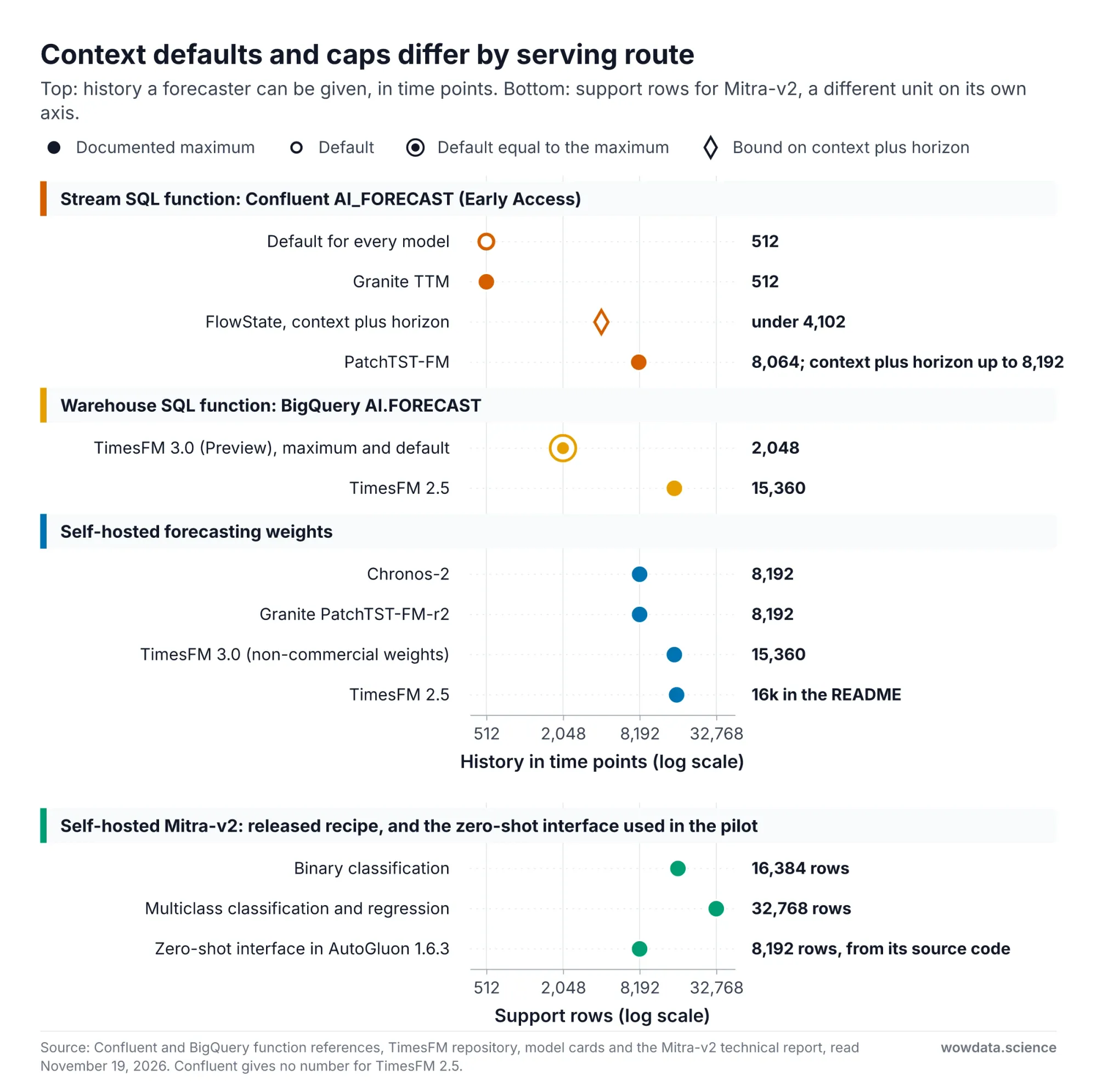
Fig 11: Documented context defaults and caps by serving route — wowdata.science
The Mitra-v2 report also lists a community DuckDB extension that runs zero-shot Mitra from SQL through ONNX. We have not tested it.
None of the managed SQL functions can run Mitra-v2 today, and their documentation offers no way to choose rows other than the most recent ones. A context policy more elaborate than "the last n points" still means an external scorer.
Advanced Data Patterns for Model Context
These seven patterns follow from the constraints above. Each is a candidate to be tested, not a recommendation.
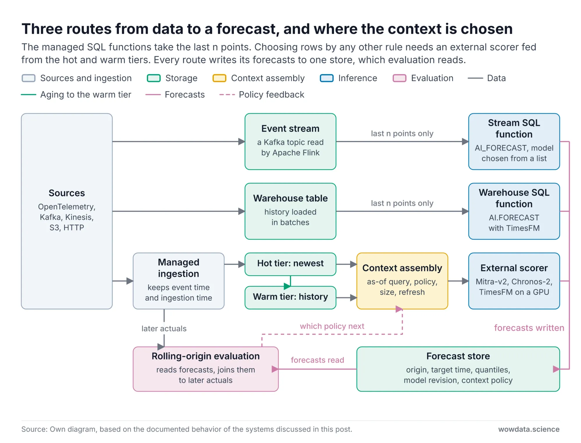
Fig 12: Three data routes from source to forecast and where context is assembled — wowdata.science
1. Point-in-time context. Every context must be reconstructible as of a forecast origin: only rows, labels and covariate values that had arrived by then. This needs two timestamps per record, event time and ingestion time, and a query that filters on both. Without it, backtests leak late-arriving data and look better than production.
2. Two-tier context. Take half of the context from the newest rows in the hot tier and half as a sample of older history from the warm tier. In our pilot, for Mitra-v2, this mixed policy was never clearly worse than a uniform sample, and it had the lowest mean log-loss of the three policies when the cutoff of a 512-row context was advanced daily. Both are exploratory observations. For LightGBM with 512 rows it had the higher mean log-loss, 1.05 against 0.92. That is one dataset.
3. Context cutoff as a parameter. How recent the context is allowed to be is a separate choice from what goes into it, and it is bounded by how quickly labels arrive. In the pilot, advancing the cutoff of a mixed 512-row context daily instead of leaving it at the origin for three weeks lowered the mean log-loss from 0.58 to 0.49, at six of eight origins, while a uniform sample barely changed. Treat the cutoff as a measured variable, and record it with every forecast.
4. Context windows as stream state. In a stream processor, the context is state. A longer context means more state per key, so context length becomes a capacity question. The 512-point default in AI_FORECAST keeps that state small. Whether it is a good statistical default depends on the model. In Pilot 2 it was too short for Chronos-2, which AI_FORECAST does not offer. For TimesFM 2.5, which it does offer, we saw no clear gain beyond it. That is one series.
5. A forecast store. Write every forecast back as its own record: series identifier, forecast origin, target time, quantile, value, model revision and context policy. With that table, rolling-origin evaluation becomes a join between forecasts and later actuals, and a model change becomes a comparison between two revisions on the same origins. In a time series collection the designated timestamp is immutable, so choose deliberately whether it holds the origin or the target time.
6. Embeddings live next door. "Have we seen this pattern before" needs a vector index. Time series collections cannot hold one, so window embeddings from a model such as TSPulse belong in a separate vector search collection, keyed back to the series and time range.
7. The tabular bridge. Recast forecasting as tabular regression with lags, calendar features and covariates, and use a tabular foundation model with a distributional head. TabPFN-TS established the approach with TabPFN, and the Mitra-v2 report cites an independent study in which Mitra was the most accurate of four base forecasters for day-ahead electricity prices. That is Amazon's summary. We did not read the study. Pilot 3 tried it with Mitra-v2.
These patterns also suggest what to ask of database teams: sampled reads from the warm tier, as-of queries as a primitive, a way to register your own model behind the SQL function, vector indexes beside time series data, and a documented schema for forecast write-back.
The Research Plan
Four decisions shape the plan. It asks for two effect sizes with intervals, not for a share of accuracy "explained by context", because such a share depends on the levels the researcher happens to choose. The thesis is stated as a hypothesis with evidence against it. The database comparison is a map of constraints, not a ranking. And every contrast is paired, repeated where inference is random, and fixed in advance.
Research Questions
RQ-T (tabular, the core study). On time-ordered tables, how large is the effect on Mitra-v2's error of changing the context policy at a fixed checkpoint, compared with the effect of swapping the checkpoint at a fixed policy?
RQ-F (forecasting). For zero-shot forecasters, how large is the effect of history length and covariate availability at a fixed model, compared with the effect of swapping models at a fixed history, and does the ranking of models change with history length?
RQ-S (systems, descriptive). Which context policies can each data system express, at what context limit, and at what measured cost and latency on a stated date?
The tight constraint is cost. One fine-tuned Mitra-v2 fit takes minutes, so that arm cannot cover many datasets. On novelty, Drift-Resilient TabPFN, LoCalPFN, TabPFN-TS and the t0 report each cover a part. We did not find a study that measures both effects for tabular and time series models under one protocol.
Hypotheses and Falsification Conditions
| Question | Hypothesis | Refuted if |
|---|---|---|
| RQ-T | At equal context size, some policy that includes recent rows lowers error relative to a uniform sample, and the gain grows with measured drift. | The upper bound of the gain is below the minimum effect, or the slope against drift is not positive. |
| RQ-T | The policy effect at a fixed checkpoint is at least as large as the checkpoint effect at a fixed policy. | The interval for policy effect minus checkpoint effect lies below zero. |
| RQ-F | Longer history lowers error until the context covers several seasonal cycles, and model rankings depend on history length. | The upper bound of the history gain is below the minimum effect, and no ranking reversal has an interval excluding zero. |
| RQ-F | With the same covariates, a tabularized Mitra-v2 regressor is within the minimum effect of the best native forecaster. | The lower bound of its excess error exceeds the minimum effect. |
| RQ-S | At least one tiering or placement choice lowers cost at equal context fidelity within the latency budget. | Every tested alternative fails fidelity or latency, or saves less than 10 percent. |
Intervals that straddle a threshold are reported as inconclusive. A non-significant difference is not treated as equivalence.
Which contrasts count. A comparison between "the policy effect" and "the model effect" can be won by choosing the contrasts after the fact. The confirmatory contrasts are therefore fixed before any test origin is opened: recent against uniform and mixed against uniform at each context size, daily against origin cutoff for each policy, the named checkpoint pairs at each policy, and the named forecaster pairs at each history length. Policy and model contrasts are compared only on inputs that every model in the pair accepts and that a deployment could serve. Results at a model's own maximum context, or beyond the context length a checkpoint was pretrained on, are analyzed separately and do not enter that comparison. The interaction between policy and model is reported, not averaged away. Before the test origins are opened, the protocol also names which matched contrasts decide the primary verdict, how their magnitudes are summarized, and how the verdict is reported for the narrow and the wide model range.
Experimental Design
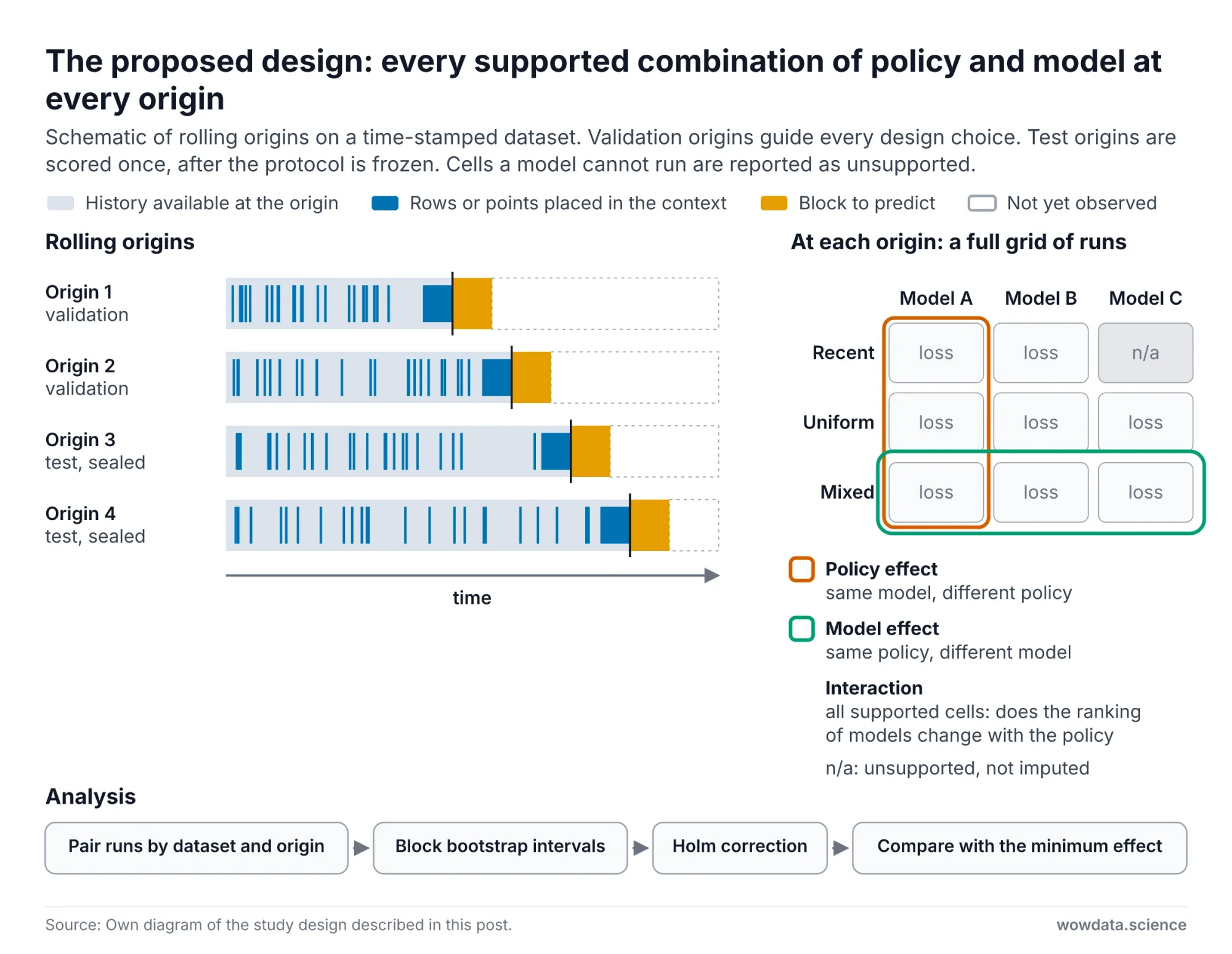
Fig 13: Crossed rolling-origin design of the proposed study — wowdata.science
| Factor | Levels | Held fixed |
|---|---|---|
| Tabular row selection | Recent, uniform, mixed, nearest neighbors per query | Context size, features, preprocessing |
| Time as a feature | No timestamp column, timestamp column added | Row selection, context size |
| Context size | 512, 2,048, 8,192, 32,768 support rows | Policy |
| Context cutoff | At the origin, advanced daily, advanced per query batch | Policy, size, scoring batches and random seeds |
| Tabular checkpoint | Mitra-v2 and Mitra-v1 zero-shot as the swap, since the classifiers share an architecture. It is clean only up to the 512 support rows Mitra-v1 was pretrained on. Mitra-v2 fine-tuned as a separate arm. A second model family, named before any test origin is opened, if it accepts identical support rows. | Policy |
| History length | 128, 512, 2,048, 8,192 points, and each model's maximum | Horizon, origins |
| Forecasting model | TimesFM 2.5 and Chronos-2 as the year-old models, Granite PatchTST-FM-r2, plus TimesFM 3.0, TimeH2O-v1 and t0 where the license allows research use | History length |
| Covariates | None, past only, past and future | Raw history |
| Baselines | Seasonal naive, AutoETS, LightGBM on the same rows, TabPFN-TS | Not applicable |
Three rules keep the comparison fair. Zero-shot and fine-tuned arms are never mixed in one contrast. Every result reports compute per forecast. And any arm with random inference is run at least three times, with the spread between runs reported beside the effect. Cells a model cannot run, such as 8,192 points for a model capped at 512, are reported as unsupported and are not imputed.
Data, Leakage and Drift
- Selection. Time-stamped, non-personal, redistributable datasets with documented availability times. Tabular data in the style of TabReD. Forecasting tasks from TIME first, because it was built from fresh datasets to resist contamination, then fev-bench and GIFT-Eval.
- Timeline. An early block for warm-up, rolling validation origins for every design decision, and later test origins that stay sealed until the protocol is frozen.
- Leakage. All preprocessing is fitted on data before each origin. Features and covariates are reconstructed as they were known at prediction time, and the availability time of every feature and label is written down per dataset. Each dataset is tagged for pretraining overlap as known, unlikely or unknown, and results are repeated without the unknown ones.
- Drift. Measured per origin without labels, as the cross-validated AUC of a classifier that separates context rows from query rows. A value of 0.5 means the classifier does no better than chance.
The evaluation rules follow the forecasting literature collected at mlpapers.org: rolling-origin evaluation, seasonal naive and automatic statistical baselines, scores matched to the forecast target, and no ranking from a single test window.
Metrics and Statistics
| Task | Primary metric | Secondary |
|---|---|---|
| Classification | Log-loss | ROC-AUC, calibration |
| Regression | RMSE | CRPS from the predictive distribution |
| Point forecasting | MASE of the median | Error by horizon |
| Probabilistic forecasting | Weighted quantile loss on shared quantiles | Interval coverage |
| Serving | Cost per on-time prediction | p50 and p95 latency, state size |
In the full study, each loss is divided by the loss of a fixed baseline on the same task and the same test windows: seasonal naive for forecasting, the class prior or the training mean for tabular tasks. The normalized losses are averaged with equal weight per dataset. Tasks with a zero or near-zero baseline loss are listed and excluded, not silently dropped. The pilot used simpler definitions, which are given with its results.
The minimum effect of interest is 0.02 in normalized loss. Uncertainty comes from a paired block bootstrap that keeps overlapping horizons and related series together. Where a contrast rests on fewer than about 20 origins, a t interval and an exact permutation test replace the bootstrap, as in Pilot 1. Pilot 2 used an ordinary bootstrap over origins, with a block bootstrap as a check. Confirmatory contrasts are corrected with the Holm procedure.
Threats to Validity
- Internal. Timestamp leakage and unequal tuning can pass for model effects. As-of joins and fixed tuning budgets address this.
- External. A small panel of datasets cannot establish a general ranking. Results are reported per dataset as well as pooled.
- Construct. More history changes compute as well as information. Runtime and retained inputs are logged for every run.
- Statistical. Overlapping origins and few datasets reduce the effective sample size. Block resampling and leave-one-dataset-out checks address this.
- Stochastic inference. Some interfaces give different predictions for the same input. Runs are seeded, repeated and averaged, and effects smaller than the spread between runs are not interpreted.
- Vendor numbers. Leaderboard snapshots motivate contrasts and are never used as results.
- Unequal ranges. A wide range of policies compared with a narrow range of models favors the hypothesis by construction. Both ranges are fixed in advance, and the comparison is reported for a narrow and a wide model range.
- Licenses. Non-commercial weights are used only where the license permits research evaluation, and that is stated per model.
Twelve-Week Schedule
| Weeks | Work |
|---|---|
| 1 to 2 | Screen datasets and licenses. Verify adapters, memory limits and SQL access. |
| 3 to 4 | Build the as-of replay and baselines. Pilot on validation origins. Freeze the protocol and register it. |
| 5 to 7 | Run the paired offline comparisons on one 24 GB GPU. Cache every prediction. |
| 8 to 10 | Run bounded cloud replays for RQ-S with billing checks. Analyze paired effects. |
| 11 to 12 | Reproduce a sample of runs from scratch. Publish code, splits, seeds, model revisions and the dates every leaderboard was read. |
If time is cut in half, the minimum study is two forecasters at two history lengths, one Mitra-v2 classification test of context policy, and external scoring against two tier settings.
Frequently Asked Questions
What are time series foundation models
Time series foundation models are neural networks pretrained on very large collections of real and synthetic series so that they can forecast a new series without being trained on it. You pass the recent history, and sometimes covariates, as context, and the model returns a point forecast or quantiles. TimesFM, Chronos-2, TimeH2O, t0 and the IBM Granite models are examples. Tabular foundation models such as Mitra-v2 do the same for tables: they predict from labeled rows placed in their context.
What is Mitra-v2
Mitra-v2 is Amazon's second-generation tabular foundation model, released on September 3, 2026, under Apache-2.0. It has a classifier with 75.7M parameters and a regressor with 76.7M. It is pretrained only on synthetic data and predicts by reading labeled rows placed in its context, without training a model per dataset.
Is Mitra-v2 zero-shot
The classifier can be used zero-shot. The published benchmark results are not zero-shot: they use a 50-step fine-tune with 8-fold bagging, which the technical report says takes a median of roughly nine minutes per evaluation unit.
Can I use TimesFM 3.0 commercially
Not with the downloaded weights. They are under a non-commercial license. Commercial use is available through authorized Google Cloud services such as BigQuery ML, which exposes TimesFM through AI.FORECAST. TimesFM 2.5 remains Apache-2.0.
Which is more accurate, TimeH2O or TimesFM 3.0
On public benchmarks in November 2026, TimeH2O-v1 is ahead by a small margin: about 2 percent in MASE and 3 percent in CRPS on GIFT-Eval, and 3.6 percent on fev-bench, with intervals that exclude zero. Those figures come from submitted results that we reaggregated, not from models that we reran. Both sets of weights are non-commercial. On your own data the difference may be smaller than the effect of how much history you provide.
How much history does a time series foundation model need
It depends on the model and on the sampling rate. In our pilot on one half-hourly electricity demand series, the comparison between 512 and 8,192 points was inconclusive for TimesFM 2.5, while for Chronos-2, 2,048 points was the shortest tested history at which it clearly beat a weekly seasonal naive forecast. On a 12-pair subset of GIFT-Eval, the t0 report finds its model within 5 percent of its full-context CRPS from a 1,024-point cap. Test several lengths on your own series before settling on a default.
What are OpenSearch Serverless time series collections
They are a collection type in the next generation of Amazon OpenSearch Serverless, announced on October 28, 2026, for logs, metrics, traces and event data. They add a lower-cost warm storage tier, retention settings up to 3,650 days, and built-in alerting and anomaly detection. OpenSearch Ingestion can write to them since November 17, 2026.
What is a streamhouse
In IBM and Confluent's usage, a streamhouse is a data streaming platform that continuously captures, processes, governs and serves current business data, with Apache Flink processing it in motion. Their time series functions run foundation models over those streams from SQL.
Can a tabular foundation model forecast time series
Yes, by turning forecasting into regression on lag and calendar features. TabPFN-TS showed this with TabPFN. In our Pilot 3, on four origins of one series, the Mitra-v2 regressor had about the same mean error as LightGBM on the same features and as a weekly seasonal naive forecast. The observed means of the native forecasters fell on both sides of it, depending on how much history they were given. Four origins do not support a ranking.
Conclusion
In late 2026 the best single-model entries are close on GIFT-Eval MASE, and the tabular boards are harder to read because vendors report results under different protocols. Those benchmarks fix the context in advance. Real deployments do not. The data platform decides how many rows, how much history and how fresh a context each model receives.
Our pilot covers one dataset and supports only a narrow statement: the largest effects we observed came from changing a small support set or extending a short forecast history. It does not establish where context stops mattering, and it was not designed to test the hypothesis.
That leaves a hypothesis with published evidence on both sides. The plan above is designed to test it properly: paired effects of context policy and model on time-ordered data, with contrasts fixed in advance, rolling origins, sealed test periods and stated ways to be wrong.
References and Further Reading
- Mitra-v2 Technical Report, Tao et al., Amazon, 2026
- Mitra-v2: Scaling synthetic pretraining for tabular foundation models, Amazon Science, November 10, 2026
- autogluon/mitra-classifier-2 model card, Hugging Face
- autogluon/mitra-regressor-2 model card, Hugging Face
- autogluon/mitra-finetune package and results, Hugging Face
- Mitra: Mixed Synthetic Priors for Enhancing Tabular Foundation Models, Zhang et al., NeurIPS 2025
- A decoder-only foundation model for time-series forecasting, Das et al., ICML 2024
- TimesFM-3: A zero-shot foundation model for multivariate forecasting, Google Research, August 31, 2026
- TimesFM repository and license notice, Google Research
- google/timesfm-3.0-pytorch model card, Hugging Face
- TimeH2O: Compact Foundation Models for Time Series Forecasting, H2O.ai, October 26, 2026
- t0: A Time-Series Foundation Model for Forecasting with Context, Meyer et al., The Forecasting Company, 2026
- Time-Series Models in the Streamhouse: A New Frontier and Use Cases, IBM Research and Confluent, November 18, 2026
- Real-Time Intelligence with IBM Time Series Models on Confluent, IBM Research, 2026
- Revisiting the Generic Transformer: Deconstructing a Strong Baseline for Time Series Foundation Models, Wen et al., 2026
- Chronos-2: From Univariate to Universal Forecasting, Ansari et al., 2025
- Toto 2.0: Time Series Forecasting Enters the Scaling Era, Khwaja et al., 2026
- TiRex: Zero-Shot Forecasting Across Long and Short Horizons, Auer et al., NeurIPS 2025
- TiRex-2: Generalizing TiRex to Multivariate Data and Streaming, Podest et al., 2026
- GIFT-Eval: A Benchmark for General Time Series Forecasting Model Evaluation, Aksu et al., 2024
- fev-bench: A Realistic Benchmark for Time Series Forecasting, Shchur et al., NeurIPS 2026
- It's TIME: Towards the Next Generation of Time Series Forecasting Benchmarks, Qiao et al., ICML 2026
- TabArena: A Living Benchmark for Machine Learning on Tabular Data, Erickson et al., NeurIPS 2025
- TALENT: A Tabular Analytics and Learning Toolbox, Liu et al., 2024
- TabPFN-3: Technical Report, Grinsztajn et al., 2026
- EXAONE Tabular 1.0: Technical Report, Eo et al., 2026
- TabFM: A Zero-Shot Foundation Model for Tabular Data, Kong et al., 2026
- TabReD: Analyzing Pitfalls and Filling the Gaps in Tabular Deep Learning Benchmarks, Rubachev et al., 2024
- Drift-Resilient TabPFN, Helli et al., NeurIPS 2024
- Retrieval and Fine-Tuning for In-Context Tabular Models, Thomas et al., 2024
- From Tables to Time: Extending TabPFN-v2 to Time Series Forecasting, Hoo et al., 2025
- Shaping the Prior: How Synthetic Task Distributions Determine Tabular Foundation Model Quality, Bouadi et al., 2026
- Time Series Forecasting: papers and methods, mlpapers.org
- Amazon OpenSearch Ingestion now supports next-generation time series collections, AWS, November 17, 2026
- Introducing time series collections for the next generation of Amazon OpenSearch Serverless, AWS, October 28, 2026
- Using the warm-after setting in time series collections, AWS documentation
- Managing data retention for NextGen time series collections, AWS documentation
- Using the timestamp field in time series collections, AWS documentation
- Configuring anomaly detection on Amazon OpenSearch Serverless, AWS documentation
- Data Prepper OpenSearch sink, OpenSearch documentation
- Forecast Data Trends with Confluent Cloud for Apache Flink, Confluent documentation
- The AI.FORECAST function, Google Cloud documentation
- The TimesFM model in BigQuery ML, Google Cloud documentation
- GIFT-Eval leaderboard and raw results, Salesforce AI Research
- fev library and fev-bench results, AutoGluon
How this post was made: it was researched, computed and drafted by an AI coding agent working under human direction, following an academic research workflow. The agent read the primary sources, recomputed GIFT-Eval and fev-bench from their raw result files, and ran the pilot (the Mitra-v2 and Mitra-v1 classifiers, the Mitra-v2 regressor, TimesFM 2.5, Chronos-2 and LightGBM) on one NVIDIA A10G on November 19, 2026, with one repeat of the Mitra-v2 and LightGBM rows of Pilot 3 a day later. It did not run the OpenSearch index template, the OpenSearch Ingestion pipeline, the Flink SQL statement or the BigQuery query shown above. It did not run TimesFM 3.0, TimeH2O or t0: their numbers here come from their publishers or from public leaderboard files. Other AI models reviewed the research plan and this post, and both were revised after those reviews. A person chose the topic, the initial sources and the tools. No person has independently repeated the experiments. Vendor figures are labeled as such. The charts are drawn with d3.js and the 3D diagram with three.js. The two animated replays, Fig 6 and Fig 8, show recorded results and summaries computed from them, and narrate them as they play, an approach borrowed from Marc Brooker's animations for system builders. The animated 3D diagram, Fig 2, is a schematic.